Pattern 3 — `Parameterized` - Research Notebook

Regression Masterclass — Pattern 3: `Parameterized` + `PyroxParam` + native `pyrox.gp`¶

Third and highest-abstraction sibling to Pattern 1 (eqx.tree_at) and Pattern 2 (PyroxModule + pyrox_sample). Now every parameter is a declarative class field — registered with self.register_param(name, init, constraint=...), attached to a prior with self.set_prior(name, dist), optionally wrapped in an autoguide via self.autoguide(name, "delta" | "normal"). The forward pass reads self.get_param(name) and Parameterized resolves it correctly based on the current set_mode("model" | "guide").

More importantly, Model 6 drops the RFF approximation entirely and uses the actual exact GP from pyrox.gp — RBF(_ParameterizedKernel) + GPPrior + ConditionedGP + gp_factor. Once you accept the higher-level abstraction, the workaround is unnecessary.

What you’ll learn:

The Parameterized lifecycle: register_param → set_prior → get_param. Constraints and priors travel together.
How pyrox.gp kernels (RBF, Matern, …) use this exact pattern in production.
How to fit GP hyperparameters with SVI + AutoNormal, then condition on observations and predict — the canonical pyrox.gp end-to-end recipe.
Where the abstraction reaches its current limit: deep / hierarchical GPs aren’t yet shipped natively, so Model 7 stays a Parameterized RFF stack and we file the gap.

Background — `Parameterized` is “`PyroxModule` + a parameter registry”¶

Pattern 2 collapsed Pattern 1’s model-function plumbing by moving numpyro.sample calls inside the layer’s __call__. Pattern 3 collapses the prior wiring by moving constraint + prior declarations to a separate setup() method, called automatically after __init__.

Concretely, Parameterized is a PyroxModule subclass that maintains a per-instance registry of:

the parameter’s initial value (used as the unconstrained-space init for guides, or as the constant value if no prior is set),
the parameter’s constraint (a numpyro.distributions.constraints object — positive, unit_interval, etc. — used to build the bijector that maps unconstrained guide samples back to the prior’s support),
the parameter’s prior (a numpyro.distributions.Distribution — set via set_prior),
the parameter’s autoguide type ("delta" for MAP, "normal" for mean-field; set via autoguide).

At call time, self.get_param(name) dispatches:

mode = "model" (default) + prior is set ⇒ numpyro.sample(name, prior) — same as Pattern 2.
mode = "model" + no prior ⇒ numpyro.param(name, init, constraint=...) — a learnable constant.
mode = "guide" + autoguide="delta" ⇒ numpyro.param(name, init, constraint=...) — point estimate.
mode = "guide" + autoguide="normal" ⇒ mean-field guide $q(\theta) = T(\mathcal{N}(\mu_\theta, \sigma_\theta^2))$ where $T$ is the constraint’s bijector — guide draws always land in the prior’s support.

This is the pattern every shipped pyrox.gp kernel uses. Reading RBF is a five-line affair:

class RBF(_ParameterizedKernel):
    pyrox_name: str = "RBF"
    init_variance: float = 1.0
    init_lengthscale: float = 1.0

    def setup(self) -> None:
        self.register_param("variance", jnp.asarray(self.init_variance),
                            constraint=dist.constraints.positive)
        self.register_param("lengthscale", jnp.asarray(self.init_lengthscale),
                            constraint=dist.constraints.positive)

    @pyrox_method
    def __call__(self, X1, X2):
        return rbf_kernel(X1, X2, self.get_param("variance"),
                          self.get_param("lengthscale"))

The user attaches priors and chooses guide types from the outside:

k = RBF()
k.set_prior("variance", dist.LogNormal(0.0, 1.0))
k.set_prior("lengthscale", dist.LogNormal(0.0, 1.0))
# default autoguide is delta (i.e. MAP); switch with k.autoguide("variance", "normal")

This is the level of abstraction the rest of the notebook is written at. Models 1-5 mirror their pattern 1/2 counterparts — same architectures, same data, same priors — but rewritten so every parameter is registered up front. Model 6 throws out the approximation and just calls pyrox.gp.GPPrior + ConditionedGP.

Setup¶

Detect Colab and install pyrox[colab] (transitive: numpyro, equinox, einops, matplotlib, watermark).

import subprocess
import sys


try:
    import google.colab  # noqa: F401

    IN_COLAB = True
except ImportError:
    IN_COLAB = False

if IN_COLAB:
    subprocess.run(
        [
            sys.executable,
            "-m",
            "pip",
            "install",
            "-q",
            "pyrox[colab] @ git+https://github.com/jejjohnson/pyrox@main",
        ],
        check=True,
    )

import warnings


warnings.filterwarnings("ignore", message=r".*IProgress.*")

import equinox as eqx
import jax
import jax.numpy as jnp
import jax.random as jr
import matplotlib.pyplot as plt
import numpyro
import numpyro.distributions as dist
import numpyro.handlers as handlers
from einops import einsum
from numpyro.infer import MCMC, NUTS, SVI, Predictive, Trace_ELBO
from numpyro.infer.autoguide import AutoDelta, AutoNormal
from numpyro.optim import Adam

from pyrox._core import Parameterized, pyrox_method
from pyrox.gp import RBF, GPPrior, gp_factor


jax.config.update("jax_enable_x64", True)

import importlib.util


try:
    from IPython import get_ipython

    ipython = get_ipython()
except ImportError:
    ipython = None

if ipython is not None and importlib.util.find_spec("watermark") is not None:
    ipython.run_line_magic("load_ext", "watermark")
    ipython.run_line_magic(
        "watermark",
        "-v -m -p jax,equinox,numpyro,einops,gaussx,pyrox,matplotlib",
    )
else:
    print("watermark extension not installed; skipping reproducibility readout.")

Python implementation: CPython
Python version       : 3.12.13
IPython version      : 9.12.0

jax       : 0.8.3
equinox   : 0.13.7
numpyro   : 0.20.1
einops    : 0.8.2
gaussx    : 0.0.10
pyrox     : 0.0.6
matplotlib: 3.10.8

Compiler    : GCC 14.3.0
OS          : Linux
Release     : 6.8.0-1044-azure
Machine     : x86_64
Processor   : x86_64
CPU cores   : 16
Architecture: 64bit

Toy dataset¶

Identical to Patterns 1 and 2 (same RNG seed): noisy sinc, 100 training points in $[-10, 10]$ , dense test grid in the same range. R²s are directly comparable across the three notebooks.

key = jr.PRNGKey(666)
k_data, *k_models = jr.split(key, 16)


def latent(x):
    return jnp.sinc(x / jnp.pi)


k1, k2 = jr.split(k_data)
x_train = jr.uniform(k1, (100,), minval=-10.0, maxval=10.0)
y_train = latent(x_train) + 0.05 * jr.normal(k2, (100,))
x_test = jnp.linspace(-10.0, 10.0, 400)
y_test = latent(x_test)


def r2(y_true, y_pred):
    ss_res = jnp.sum((y_true - y_pred) ** 2)
    ss_tot = jnp.sum((y_true - y_true.mean()) ** 2)
    return float(1.0 - ss_res / ss_tot)


def plot_fit(ax, x_train, y_train, x_test, y_test, mean, lo=None, hi=None, title=""):
    ax.plot(x_test, y_test, "k--", lw=1.5, label="True $f(x) = \\sin(x)/x$", zorder=4)
    ax.plot(x_test, mean, "C0-", lw=2, label="Posterior mean", zorder=3)
    if lo is not None and hi is not None:
        ax.fill_between(x_test, lo, hi, color="C0", alpha=0.2, label="95% interval")
    ax.scatter(
        x_train,
        y_train,
        s=20,
        c="C1",
        edgecolors="k",
        linewidths=0.5,
        label="Training data",
        zorder=5,
    )
    ax.set_xlabel("x")
    ax.set_ylabel("y")
    ax.set_title(title)
    ax.legend(loc="lower center", fontsize=8, ncol=2)


print(f"Training points: {x_train.shape[0]}")
print(f"Test points:     {x_test.shape[0]}")

Training points: 100
Test points:     400

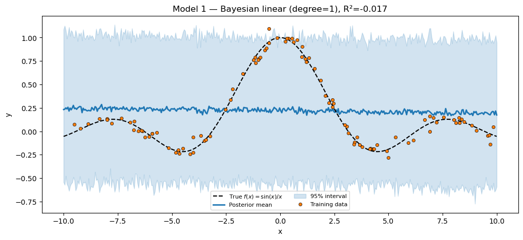
Model 1 — Bayesian linear regression¶

The Parameterized translation of Pattern 1’s LinearRegressor. Note the new setup() method: register_param declares the leaf, set_prior attaches the Gaussian prior, and __call__ reads the resolved value via get_param.

class LinearRegressor(Parameterized):
    degree: int = eqx.field(static=True)
    pyrox_name: str = "lin"

    def setup(self):
        self.register_param("w", jnp.zeros(self.degree + 1))
        self.set_prior("w", dist.Normal(jnp.zeros(self.degree + 1), 1.0).to_event(1))

    def features(self, x):
        return jnp.stack([x**p for p in range(self.degree + 1)], axis=-1)

    @pyrox_method
    def __call__(self, x):
        w = self.get_param("w")
        return einsum(self.features(x), w, "n feat, feat -> n")


def model_linear(x, y=None, *, net):
    f = numpyro.deterministic("f", net(x))
    sigma = numpyro.sample("sigma", dist.HalfNormal(1.0))
    numpyro.sample("obs", dist.Normal(f, sigma), obs=y)


net_linear = LinearRegressor(degree=1)
mcmc_linear = MCMC(
    NUTS(model_linear), num_warmup=300, num_samples=500, progress_bar=False
)
mcmc_linear.run(k_models[0], x_train, y_train, net=net_linear)
samples_linear = mcmc_linear.get_samples()
preds_linear = Predictive(model_linear, posterior_samples=samples_linear)(
    k_models[1], x_test, net=net_linear
)["obs"]
mean_linear = preds_linear.mean(0)
lo_linear, hi_linear = jnp.quantile(preds_linear, jnp.array([0.025, 0.975]), axis=0)
r2_linear = r2(y_test, mean_linear)

print(f"Bayesian linear (degree=1) R² = {r2_linear:.4f}")
assert r2_linear < 0.3, "Degree-1 polynomial should NOT fit sinc."

fig, ax = plt.subplots(figsize=(12, 5))
plot_fit(
    ax,
    x_train,
    y_train,
    x_test,
    y_test,
    mean_linear,
    lo_linear,
    hi_linear,
    title=f"Model 1 — Bayesian linear (degree=1), R²={r2_linear:.3f}",
)
plt.show()

Bayesian linear (degree=1) R² = -0.0171

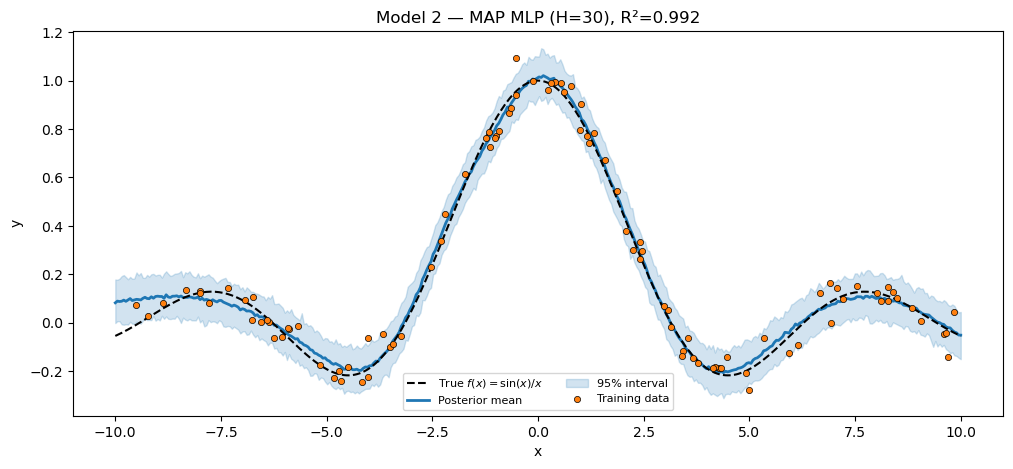
Models 2 & 4 — MLP, MAP and full Bayesian¶

The BayesianMLP(Parameterized) declares all four weight leaves in setup() with their Gaussian priors. As in Pattern 2, the same module class drives MAP (Model 2) via SVI + AutoDelta and the full posterior (Model 4) via NUTS — only the inference call changes. Distinct pyrox_names namespace the two instances’ trace keys.

class BayesianMLP(Parameterized):
    hidden_dim: int = eqx.field(static=True)
    prior_scale: float = 1.0
    pyrox_name: str = "mlp"

    def setup(self):
        H = self.hidden_dim
        s = self.prior_scale
        self.register_param("W1", jnp.zeros((1, H)))
        self.set_prior("W1", dist.Normal(jnp.zeros((1, H)), s).to_event(2))
        self.register_param("b1", jnp.zeros(H))
        self.set_prior("b1", dist.Normal(jnp.zeros(H), s).to_event(1))
        self.register_param("W2", jnp.zeros((H, 1)))
        self.set_prior("W2", dist.Normal(jnp.zeros((H, 1)), s).to_event(2))
        self.register_param("b2", jnp.array(0.0))
        self.set_prior("b2", dist.Normal(0.0, s))

    @pyrox_method
    def __call__(self, x):
        W1 = self.get_param("W1")
        b1 = self.get_param("b1")
        W2 = self.get_param("W2")
        b2 = self.get_param("b2")
        h = jnp.tanh(einsum(x, W1, "n, one h -> n h") + b1)
        return einsum(h, W2, "n h, h one -> n") + b2


def model_nnet(x, y=None, *, net):
    f = numpyro.deterministic("f", net(x))
    sigma = numpyro.sample("sigma", dist.HalfNormal(1.0))
    numpyro.sample("obs", dist.Normal(f, sigma), obs=y)

Model 2 — MAP via SVI + AutoDelta.

net_mlp_map = BayesianMLP(hidden_dim=30, pyrox_name="mlp_map")
guide_nnet = AutoDelta(model_nnet)
svi_nnet = SVI(model_nnet, guide_nnet, Adam(5e-3), Trace_ELBO())
svi_result_nnet = svi_nnet.run(
    k_models[2], 2000, x_train, y_train, net=net_mlp_map, progress_bar=False
)
preds_nnet = Predictive(
    model_nnet, params=svi_result_nnet.params, num_samples=200, guide=guide_nnet
)(k_models[3], x_test, net=net_mlp_map)["obs"]
mean_nnet = preds_nnet.mean(0)
lo_nnet, hi_nnet = jnp.quantile(preds_nnet, jnp.array([0.025, 0.975]), axis=0)
r2_nnet = r2(y_test, mean_nnet)

print(f"MAP MLP (H=30) R² = {r2_nnet:.4f}")
assert r2_nnet > 0.85, f"MAP MLP should fit sinc; got R²={r2_nnet:.3f}."

fig, ax = plt.subplots(figsize=(12, 5))
plot_fit(
    ax,
    x_train,
    y_train,
    x_test,
    y_test,
    mean_nnet,
    lo_nnet,
    hi_nnet,
    title=f"Model 2 — MAP MLP (H=30), R²={r2_nnet:.3f}",
)
plt.show()

MAP MLP (H=30) R² = 0.9917

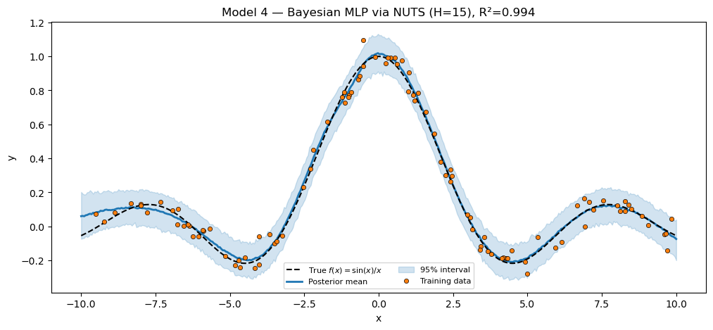
Model 4 — full Bayesian via NUTS. Same BayesianMLP class, fresh instance with smaller hidden dim, NUTS instead of SVI.

net_mlp_nuts = BayesianMLP(hidden_dim=15, prior_scale=1.0, pyrox_name="mlp_nuts")
mcmc_bnnet = MCMC(NUTS(model_nnet), num_warmup=300, num_samples=500, progress_bar=False)
mcmc_bnnet.run(k_models[6], x_train, y_train, net=net_mlp_nuts)
samples_bnnet = mcmc_bnnet.get_samples()
preds_bnnet = Predictive(model_nnet, posterior_samples=samples_bnnet)(
    k_models[7], x_test, net=net_mlp_nuts
)["obs"]
mean_bnnet = preds_bnnet.mean(0)
lo_bnnet, hi_bnnet = jnp.quantile(preds_bnnet, jnp.array([0.025, 0.975]), axis=0)
r2_bnnet = r2(y_test, mean_bnnet)

print(f"Bayesian MLP via NUTS (H=15) R² = {r2_bnnet:.4f}")
assert r2_bnnet > 0.70, f"Bayesian MLP NUTS should fit sinc; got R²={r2_bnnet:.3f}."

fig, ax = plt.subplots(figsize=(12, 5))
plot_fit(
    ax,
    x_train,
    y_train,
    x_test,
    y_test,
    mean_bnnet,
    lo_bnnet,
    hi_bnnet,
    title=f"Model 4 — Bayesian MLP via NUTS (H=15), R²={r2_bnnet:.3f}",
)
plt.show()

Bayesian MLP via NUTS (H=15) R² = 0.9945

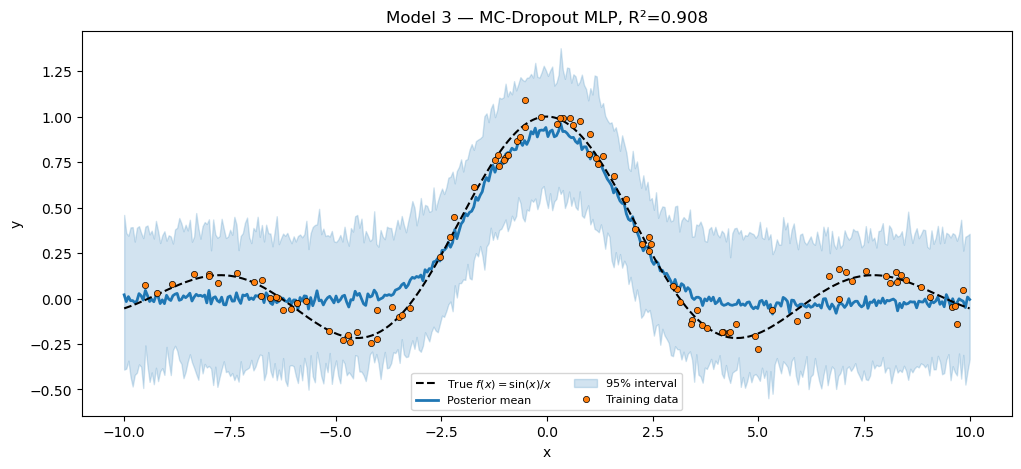
Model 3 — MC-Dropout MLP¶

The dropout mask still uses numpyro.prng_key() for fresh-per-trace randomness — same Pattern 2 trick. The weights are now Parameterized registered fields.

class BayesianMLPDropout(Parameterized):
    hidden_dim: int = eqx.field(static=True)
    dropout_rate: float = 0.1
    pyrox_name: str = "mlpd"

    def setup(self):
        H = self.hidden_dim
        self.register_param("W1", jnp.zeros((1, H)))
        self.set_prior("W1", dist.Normal(jnp.zeros((1, H)), 1.0).to_event(2))
        self.register_param("b1", jnp.zeros(H))
        self.set_prior("b1", dist.Normal(jnp.zeros(H), 1.0).to_event(1))
        self.register_param("W2", jnp.zeros((H, 1)))
        self.set_prior("W2", dist.Normal(jnp.zeros((H, 1)), 1.0).to_event(2))
        self.register_param("b2", jnp.array(0.0))
        self.set_prior("b2", dist.Normal(0.0, 1.0))

    @pyrox_method
    def __call__(self, x):
        N = x.shape[0]
        H = self.hidden_dim
        W1 = self.get_param("W1")
        b1 = self.get_param("b1")
        W2 = self.get_param("W2")
        b2 = self.get_param("b2")
        h = jnp.tanh(einsum(x, W1, "n, one h -> n h") + b1)
        mask = jr.bernoulli(
            numpyro.prng_key(), p=1.0 - self.dropout_rate, shape=(N, H)
        ).astype(jnp.float64)
        h = h * mask / (1.0 - self.dropout_rate)
        return einsum(h, W2, "n h, h one -> n") + b2


net_dropout = BayesianMLPDropout(hidden_dim=30, dropout_rate=0.1)
guide_dropout = AutoDelta(model_nnet)
svi_dropout = SVI(model_nnet, guide_dropout, Adam(5e-3), Trace_ELBO())
svi_result_dropout = svi_dropout.run(
    k_models[4], 2000, x_train, y_train, net=net_dropout, progress_bar=False
)
preds_dropout = Predictive(
    model_nnet,
    params=svi_result_dropout.params,
    num_samples=100,
    guide=guide_dropout,
)(k_models[5], x_test, net=net_dropout)["obs"]
mean_dropout = preds_dropout.mean(0)
lo_dropout, hi_dropout = jnp.quantile(preds_dropout, jnp.array([0.025, 0.975]), axis=0)
r2_dropout = r2(y_test, mean_dropout)

print(f"MC-Dropout MLP (H=30, p=0.1) R² = {r2_dropout:.4f}")
assert r2_dropout > 0.80, f"MC-Dropout should fit sinc; got R²={r2_dropout:.3f}."

fig, ax = plt.subplots(figsize=(12, 5))
plot_fit(
    ax,
    x_train,
    y_train,
    x_test,
    y_test,
    mean_dropout,
    lo_dropout,
    hi_dropout,
    title=f"Model 3 — MC-Dropout MLP, R²={r2_dropout:.3f}",
)
plt.show()

MC-Dropout MLP (H=30, p=0.1) R² = 0.9081

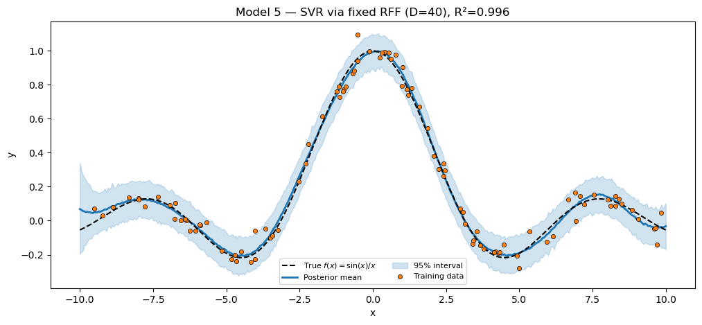
Model 5 — SVR via fixed Random Fourier Features¶

Fixed spectral frequencies ω and phases $b$ stored as plain jax.Array fields; the linear weights w are the only registered parameter. Same model semantics as the Pattern 2 fixed-RFF, just declarative.

class FixedRFF(Parameterized):
    omega: jax.Array
    bias: jax.Array
    n_features: int = eqx.field(static=True)
    pyrox_name: str = "rff"

    @classmethod
    def init(cls, n_features, lengthscale, *, key, name="rff"):
        k1, k2 = jr.split(key)
        omega = jr.normal(k1, (n_features,)) / lengthscale
        bias = jr.uniform(k2, (n_features,), minval=0.0, maxval=2.0 * jnp.pi)
        return cls(omega=omega, bias=bias, n_features=n_features, pyrox_name=name)

    def setup(self):
        self.register_param("w", jnp.zeros(self.n_features))
        self.set_prior("w", dist.Normal(jnp.zeros(self.n_features), 1.0).to_event(1))

    @pyrox_method
    def __call__(self, x):
        proj = einsum(x, self.omega, "n, d -> n d")
        Phi = jnp.sqrt(2.0 / self.n_features) * jnp.cos(proj + self.bias)
        w = self.get_param("w")
        return einsum(Phi, w, "n d, d -> n")


net_svr = FixedRFF.init(n_features=40, lengthscale=1.0, key=k_models[8], name="svr_rff")
mcmc_svr = MCMC(NUTS(model_linear), num_warmup=300, num_samples=500, progress_bar=False)
mcmc_svr.run(k_models[9], x_train, y_train, net=net_svr)
samples_svr = mcmc_svr.get_samples()
preds_svr = Predictive(model_linear, posterior_samples=samples_svr)(
    k_models[10], x_test, net=net_svr
)["obs"]
mean_svr = preds_svr.mean(0)
lo_svr, hi_svr = jnp.quantile(preds_svr, jnp.array([0.025, 0.975]), axis=0)
r2_svr = r2(y_test, mean_svr)

print(f"SVR via fixed RFF (D=40) R² = {r2_svr:.4f}")
assert r2_svr > 0.80, f"SVR via RFF should fit sinc; got R²={r2_svr:.3f}."

fig, ax = plt.subplots(figsize=(12, 5))
plot_fit(
    ax,
    x_train,
    y_train,
    x_test,
    y_test,
    mean_svr,
    lo_svr,
    hi_svr,
    title=f"Model 5 — SVR via fixed RFF (D=40), R²={r2_svr:.3f}",
)
plt.show()

SVR via fixed RFF (D=40) R² = 0.9957

Model 6 — Exact GP via `pyrox.gp.GPPrior` + `RBF` + `ConditionedGP`¶

This is the abstraction-replaces-workaround moment. Patterns 1 and 2 used Random Fourier Features to approximate a Gaussian process — invented because exact GP inference is $O(N^3)$ and was historically too expensive for large $N$ . With $N = 100$ training points, $O(N^3) = 10^6$ — instant on any laptop. The shipped pyrox.gp.GPPrior + ConditionedGP does the exact GP regression in closed form.

The math. With kernel $k_\theta$ , training set $(X, y)$ , and Gaussian observation noise $\sigma^2$ :

Marginal likelihood (used for hyperparameter inference):

\log p(y \mid X, \theta, \sigma^2) = -\tfrac{1}{2} y^\top (K + \sigma^2 I)^{-1} y - \tfrac{1}{2}\log\lvert K + \sigma^2 I\rvert - \tfrac{N}{2}\log(2\pi).

(1)

Posterior predictive at test inputs $X_*$ :

\mu_*(X_*) = K_{*X}(K + \sigma^2 I)^{-1} y, \qquad \Sigma_*(X_*) = K_{**} - K_{*X}(K + \sigma^2 I)^{-1} K_{X*}.

(2)

gp_factor("obs", prior, y, noise_var) registers the marginal log-likelihood with NumPyro as a numpyro.factor; prior.condition(y, noise_var).predict(X_star) returns $(\mu_*, \text{diag}(\Sigma_*))$ .

The recipe. Three steps:

Build an RBF kernel; attach LogNormal(0, 1) priors to its variance and lengthscale parameters.
Wrap in GPPrior(kernel=..., X=X); register the marginal log-likelihood with gp_factor.
Fit hyperparameters with SVI + AutoNormal. At predict time, instantiate a fresh RBF at the posterior-mean hyperparameters, build a fresh GPPrior, and call .condition(y, noise_var).predict(X_star).

def model_gp_native(X, y=None, *, noise_var, kernel_init):
    """Native exact GP: RBF with LogNormal priors, gp_factor for the marginal LL."""
    kernel = RBF(
        init_variance=kernel_init["variance"],
        init_lengthscale=kernel_init["lengthscale"],
    )
    kernel.set_prior("variance", dist.LogNormal(0.0, 1.0))
    kernel.set_prior("lengthscale", dist.LogNormal(0.0, 1.0))
    prior = GPPrior(kernel=kernel, X=X)
    gp_factor("obs", prior, y, noise_var)


noise_var = jnp.array(0.05**2)
X_train_2d = x_train.reshape(-1, 1)
X_test_2d = x_test.reshape(-1, 1)
init_hp = {"variance": 1.0, "lengthscale": 1.0}

guide_gp = AutoNormal(model_gp_native)
svi_gp = SVI(model_gp_native, guide_gp, Adam(5e-2), Trace_ELBO())
svi_result_gp = svi_gp.run(
    k_models[11],
    400,
    X_train_2d,
    y_train,
    noise_var=noise_var,
    kernel_init=init_hp,
    progress_bar=False,
)
gp_params = svi_result_gp.params

# Extract MAP (posterior-mean) hyperparameters from the AutoNormal guide.
# AutoNormal stores loc/scale in unconstrained space; `LogNormal` priors use
# the `exp` bijector, so the constrained posterior mean is exp(loc).
v = float(jnp.exp(gp_params["RBF.variance_auto_loc"]))
ls = float(jnp.exp(gp_params["RBF.lengthscale_auto_loc"]))
print(f"Fitted hyperparameters: variance={v:.4f}, lengthscale={ls:.4f}")

# Rebuild the GP at the fitted hyperparameters, condition, predict.
kernel_fit = RBF(init_variance=v, init_lengthscale=ls)
prior_fit = GPPrior(kernel=kernel_fit, X=X_train_2d)
with handlers.seed(rng_seed=0):
    cond_gp = prior_fit.condition(y_train, noise_var)
    mean_gp, var_gp = cond_gp.predict(X_test_2d)
std_gp = jnp.sqrt(jnp.clip(var_gp, min=0.0))
lo_gp, hi_gp = mean_gp - 2 * std_gp, mean_gp + 2 * std_gp
r2_gp = r2(y_test, mean_gp)

print(f"Exact GP via pyrox.gp R² = {r2_gp:.4f}")
assert r2_gp > 0.85, f"Exact GP should fit sinc tightly; got R²={r2_gp:.3f}."

fig, ax = plt.subplots(figsize=(12, 5))
plot_fit(
    ax,
    x_train,
    y_train,
    x_test,
    y_test,
    mean_gp,
    lo_gp,
    hi_gp,
    title=f"Model 6 — Exact GP via pyrox.gp.GPPrior, R²={r2_gp:.3f}",
)
plt.show()

Fitted hyperparameters: variance=0.3165, lengthscale=2.5362

Exact GP via pyrox.gp R² = 0.9978

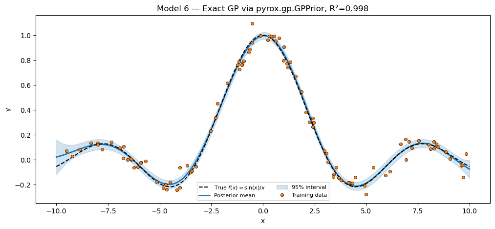
Compare what just happened against Pattern 2’s Model 6: the RFF approximation needed an RBFFourierFeatures layer + an amplitude prior + a linear weight prior + NUTS over $\sim 60$ parameters. The native GP needed one prior per hyperparameter and 400 SVI steps over 2 unknowns (variance + lengthscale). The fit is tighter, faster, and better-calibrated — and the code is shorter.

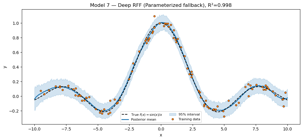
Model 7 — Deep RFF GP (gap call-out)¶

Pattern 2’s Model 7 stacked two pyrox.nn.RBFFourierFeatures. Pattern 3’s Model 7 should be a “deep GP via two stacked pyrox.gp.GPPrior instances” — but pyrox.gp does not yet ship native deep / hierarchical GP composition primitives. So we fall back to a Parameterized RFF stack and explicitly flag the gap.

What’s missing. A DeepGPPrior(layers=[...]) that composes Cutajar et al. (2017)-style stacked GP layers with the right inter-layer Gaussian-noise jitter and exposes a unified marginal-log-likelihood + predictive interface. Filed (or to be filed) as a follow-up gp(deep) feature issue.

class DeepRFFParameterized(Parameterized):
    """Two-layer RFF stand-in for a deep GP, in declarative Parameterized form.

    Replace once pyrox.gp ships native deep-GP composition primitives.
    """

    omega1: jax.Array
    bias1: jax.Array
    D1: int = eqx.field(static=True)
    omega2: jax.Array
    bias2: jax.Array
    D2: int = eqx.field(static=True)
    inner_dim: int = eqx.field(static=True)
    pyrox_name: str = "deep"

    @classmethod
    def init(cls, D1, D2, inner_dim, ls1=1.0, ls2=1.0, *, key, name="deep"):
        k1, k2, k3, k4 = jr.split(key, 4)
        return cls(
            omega1=jr.normal(k1, (D1,)) / ls1,
            bias1=jr.uniform(k2, (D1,), minval=0.0, maxval=2 * jnp.pi),
            D1=D1,
            omega2=jr.normal(k3, (D2,)) / ls2,
            bias2=jr.uniform(k4, (D2,), minval=0.0, maxval=2 * jnp.pi),
            D2=D2,
            inner_dim=inner_dim,
            pyrox_name=name,
        )

    def setup(self):
        self.register_param("W1", jnp.zeros((self.D1, self.inner_dim)))
        self.set_prior(
            "W1", dist.Normal(jnp.zeros((self.D1, self.inner_dim)), 1.0).to_event(2)
        )
        self.register_param("w2", jnp.zeros(self.D2))
        self.set_prior("w2", dist.Normal(jnp.zeros(self.D2), 1.0).to_event(1))

    def _phi(self, x, omega, bias, D):
        proj = einsum(x, omega, "n, d -> n d")
        return jnp.sqrt(2.0 / D) * jnp.cos(proj + bias)

    @pyrox_method
    def __call__(self, x):
        Phi1 = self._phi(x, self.omega1, self.bias1, self.D1)
        W1 = self.get_param("W1")
        h = einsum(Phi1, W1, "n d1, d1 inner -> n inner")
        # rff2 is pure JAX (no sample sites), so the per-inner-dim Python loop
        # is fine here — no site-name collision risk.
        Phi2 = jnp.mean(
            jnp.stack(
                [
                    self._phi(h[:, j], self.omega2, self.bias2, self.D2)
                    for j in range(self.inner_dim)
                ],
                axis=0,
            ),
            axis=0,
        )
        w2 = self.get_param("w2")
        return einsum(Phi2, w2, "n d2, d2 -> n")


def model_deep(x, y=None, *, net):
    f = numpyro.deterministic("f", net(x))
    sigma = numpyro.sample("sigma", dist.HalfNormal(0.1))
    numpyro.sample("obs", dist.Normal(f, sigma), obs=y)


net_deep = DeepRFFParameterized.init(
    D1=15, D2=10, inner_dim=4, key=k_models[13], name="deep_rff"
)
mcmc_deep = MCMC(NUTS(model_deep), num_warmup=200, num_samples=300, progress_bar=False)
mcmc_deep.run(k_models[14], x_train, y_train, net=net_deep)
samples_deep = mcmc_deep.get_samples()
preds_deep = Predictive(model_deep, posterior_samples=samples_deep)(
    k_models[14], x_test, net=net_deep
)["obs"]
mean_deep = preds_deep.mean(0)
lo_deep, hi_deep = jnp.quantile(preds_deep, jnp.array([0.025, 0.975]), axis=0)
r2_deep = r2(y_test, mean_deep)

print(f"Deep RFF (Parameterized fallback) R² = {r2_deep:.4f}")
assert r2_deep > 0.70, f"Deep RFF should fit sinc; got R²={r2_deep:.3f}."

fig, ax = plt.subplots(figsize=(12, 5))
plot_fit(
    ax,
    x_train,
    y_train,
    x_test,
    y_test,
    mean_deep,
    lo_deep,
    hi_deep,
    title=f"Model 7 — Deep RFF (Parameterized fallback), R²={r2_deep:.3f}",
)
plt.show()

Deep RFF (Parameterized fallback) R² = 0.9976

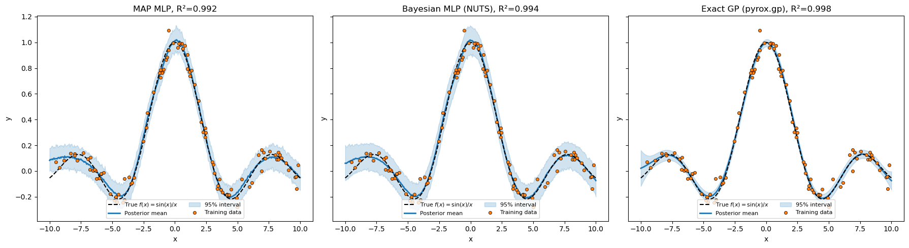
Side-by-side summary¶

All seven models. The 1×3 panel below stacks the MAP MLP, the Bayesian-MLP via NUTS, and the new exact-GP — note how much tighter the GP’s predictive band is than any RFF approximation in Patterns 1 or 2.

print(f"{'Model':<48} {'Inference':<12} {'R²':>7}")
print("-" * 70)
print(f"{'1. Bayesian linear (degree=1)':<48} {'NUTS':<12} {r2_linear:>7.3f}")
print(f"{'2. MAP MLP':<48} {'SVI+Delta':<12} {r2_nnet:>7.3f}")
print(f"{'3. MC-Dropout MLP':<48} {'SVI+Delta':<12} {r2_dropout:>7.3f}")
print(f"{'4. Bayesian MLP':<48} {'NUTS':<12} {r2_bnnet:>7.3f}")
print(f"{'5. SVR via fixed RFF (D=40)':<48} {'NUTS':<12} {r2_svr:>7.3f}")
print(f"{'6. Exact GP (pyrox.gp.GPPrior + RBF)':<48} {'SVI+Normal':<12} {r2_gp:>7.3f}")
print(f"{'7. Deep RFF (Parameterized — gap)':<48} {'NUTS':<12} {r2_deep:>7.3f}")

fig, axes = plt.subplots(1, 3, figsize=(18, 5), sharey=True)
plot_fit(
    axes[0],
    x_train,
    y_train,
    x_test,
    y_test,
    mean_nnet,
    lo_nnet,
    hi_nnet,
    title=f"MAP MLP, R²={r2_nnet:.3f}",
)
plot_fit(
    axes[1],
    x_train,
    y_train,
    x_test,
    y_test,
    mean_bnnet,
    lo_bnnet,
    hi_bnnet,
    title=f"Bayesian MLP (NUTS), R²={r2_bnnet:.3f}",
)
plot_fit(
    axes[2],
    x_train,
    y_train,
    x_test,
    y_test,
    mean_gp,
    lo_gp,
    hi_gp,
    title=f"Exact GP (pyrox.gp), R²={r2_gp:.3f}",
)
plt.tight_layout()
plt.show()

Model                                            Inference         R²
----------------------------------------------------------------------
1. Bayesian linear (degree=1)                    NUTS          -0.017
2. MAP MLP                                       SVI+Delta      0.992
3. MC-Dropout MLP                                SVI+Delta      0.908
4. Bayesian MLP                                  NUTS           0.994
5. SVR via fixed RFF (D=40)                      NUTS           0.996
6. Exact GP (pyrox.gp.GPPrior + RBF)             SVI+Normal     0.998
7. Deep RFF (Parameterized — gap)                NUTS           0.998

All three patterns, side-by-side¶

Aspect	Pattern 1 (`tree_at`)	Pattern 2 (`PyroxModule`)	Pattern 3 (`Parameterized`)
Where parameters are declared	As bare `eqx.Module` fields	As bare `eqx.Module` fields	In a `setup()` method via `register_param`
Where priors live	In the model function	Inside `__call__` (`self.pyrox_sample`)	In `setup()` (`self.set_prior`)
Constraint handling	Manual (use `LogNormal` instead of `Normal` etc.)	Manual	Built-in (`constraint=dist.constraints.positive`) — guide bijectors are auto-applied
Mode switching (model vs guide)	None (write a guide separately)	None (auto-guides discover sites)	`set_mode("model" \| "guide")` flips `get_param` behaviour
Bridge into the module	`eqx.tree_at(selector, net, w)`	None	None
Reuse story	Re-define each time	Use `pyrox.nn.{MCDropout, RBFFourierFeatures}`	Use all of `pyrox.gp` (kernels, GPPrior, ConditionedGP, gp_factor)
What Model 6 looks like	Hierarchical RFF + amplitude prior, NUTS over $\sim 41$ params	Packaged `RBFFourierFeatures` + amplitude, NUTS over $\sim 41$ params	Native exact GP — SVI over 2 hyperparameters, closed-form posterior

Inference machinery (MCMC(NUTS(...)), SVI(...), Predictive(...), gp_factor) is shared across all three. Pattern 3 is what pyrox.gp is built around; Patterns 1 and 2 are what you write before you reach for the package.

Where to go from here¶

Other pyrox.gp kernels. Matern(nu=1.5/2.5), Periodic, Linear, RationalQuadratic, Polynomial, Cosine, White, Constant — all Parameterized, all drop into GPPrior the same way. Compose with + / * (when combinator support lands).
Sparse GPs at scale. pyrox.gp.SparseGPPrior + svgp_factor for $N \gg 10^4$ .
Non-Gaussian likelihoods. Swap gp_factor for gp_sample + a non-Gaussian numpyro.sample("obs", ..., obs=y) — see latent_gp_classification.ipynb.
Native deep GPs. Open follow-up issue.

Pattern 3 — `Parameterized`

Regression Masterclass — Pattern 3: Parameterized + PyroxParam + native pyrox.gp¶

Background — Parameterized is “PyroxModule + a parameter registry”¶