GP with Uncertain Inputs (PILCO-style)

When a Gaussian process (GP) is queried at an uncertain input $x_* \sim \mathcal{N}(\mu_*, \Sigma_*)$ , the predictive distribution $p(f(x_*))$ is no longer Gaussian -- it is a mixture of Gaussians weighted by the input density. Approximating this distribution is central to several important models:

Multi-step dynamics prediction (Girard et al., 2003): the GP predicts the next state, and that uncertain prediction becomes the input for the following step. Uncertainty compounds.
PILCO (Deisenroth & Rasmussen, 2011): a GP dynamics model is rolled forward under a policy, and the expected cost is differentiated through the uncertain predictions to learn the policy.
Bayesian GPLVM (Titsias & Lawrence, 2010): latent inputs are uncertain, so the likelihood requires integrating the GP over the variational posterior of the inputs.
Heteroscedastic / input-noise GPs (McHutchon & Rasmussen, 2011): noisy inputs induce effective output noise that depends on the local gradient of the GP mean.

Predictive moments¶

Given the GP posterior $f \mid \mathcal{D}$ with weights $\alpha = (K + \sigma^2 I)^{-1} y$ and an uncertain input $x_* \sim \mathcal{N}(\mu_*, \Sigma_*)$ , the predictive moments are

\mathbb{E}[f(x_*)] = \int \mathbf{k}(x_*)^\top \alpha \;\mathcal{N}(x_* \mid \mu_*, \Sigma_*)\,dx_*,

((1))

\mathrm{Var}[f(x_*)] = \int \bigl(f(x_*) - \mathbb{E}[f(x_*)]\bigr)^2 \;\mathcal{N}(x_* \mid \mu_*, \Sigma_*)\,dx_*.

((2))

For the squared-exponential kernel, these integrals have closed-form solutions. For general kernels, we need numerical integration -- and that is where gaussx’s uncertainty propagation machinery comes in.

What this notebook covers¶

Training a 1D GP on $\sin(x)$ data
Single uncertain prediction with Taylor, Unscented, and MC methods
Multi-step dynamics rollout (PILCO-style) with growing uncertainty
Expected cost computation under input uncertainty
Expectation utilities: mean, gradient, and log-likelihood expectations
AssumedDensityFilter diagnostics: skewness, kurtosis, Gaussianity

from __future__ import annotations

import warnings


warnings.filterwarnings("ignore", message=r".*IProgress.*")

import jax
import jax.numpy as jnp
import jax.random as jr
import lineax as lx
import matplotlib.pyplot as plt

import gaussx


jax.config.update("jax_enable_x64", True)

1. Setup: 1D GP regression on sin(x)¶

We train a standard GP with an RBF kernel on noisy observations of $\sin(x)$ , then extract the weight vector $\alpha = K^{-1} y$ and the inverse kernel operator $K^{-1}$ .

key = jr.PRNGKey(42)
n_train = 40
noise_var = 0.04

# Training data
key, subkey = jr.split(key)
X_train = jr.uniform(subkey, (n_train, 1), minval=-4.0, maxval=4.0)
y_train = jnp.sin(X_train[:, 0]) + jnp.sqrt(noise_var) * jr.normal(key, (n_train,))

RBF kernel¶

lengthscale = 1.0
variance = 1.0


def rbf_kernel(x1, x2):
    """Scalar RBF kernel: (D,), (D,) -> scalar."""
    sq_dist = jnp.sum((x1 - x2) ** 2)
    return variance * jnp.exp(-0.5 * sq_dist / lengthscale**2)


# Build the kernel matrix K(X_train, X_train) + noise * I
def kernel_matrix(X):
    """Compute the full kernel matrix for training points."""
    n = X.shape[0]
    K = jax.vmap(lambda x1: jax.vmap(lambda x2: rbf_kernel(x1, x2))(X))(X)
    return K + noise_var * jnp.eye(n)


K_noisy = kernel_matrix(X_train)
K_op = lx.MatrixLinearOperator(K_noisy, lx.positive_semidefinite_tag)

# Solve for alpha = K^{-1} y
alpha = gaussx.solve(K_op, y_train)

# K_inv operator (needed for predictive variance)
K_inv = lx.MatrixLinearOperator(jnp.linalg.inv(K_noisy), lx.positive_semidefinite_tag)

Quick sanity check: plot the GP posterior at deterministic test points.

x_grid = jnp.linspace(-5, 5, 300)


def gp_predict_scalar(x_star):
    """Standard GP prediction at a single point. (D,) -> (mean, var)."""
    k_star = jax.vmap(lambda xi: rbf_kernel(x_star, xi))(X_train)
    mu = jnp.dot(k_star, alpha)
    solved = lx.linear_solve(K_op, k_star).value
    v = rbf_kernel(x_star, x_star) - jnp.dot(k_star, solved)
    return mu, jnp.maximum(v, 0.0)


mu_grid, var_grid = jax.vmap(gp_predict_scalar)(x_grid[:, None])
std_grid = jnp.sqrt(var_grid)

fig, ax = plt.subplots(figsize=(10, 4))
ax.fill_between(
    x_grid,
    mu_grid - 2 * std_grid,
    mu_grid + 2 * std_grid,
    alpha=0.2,
    color="steelblue",
)
ax.plot(x_grid, mu_grid, "steelblue", lw=2, label="GP mean", zorder=3)
ax.plot(x_grid, jnp.sin(x_grid), "k--", lw=1.5, label="sin(x)", zorder=4)
ax.scatter(
    X_train[:, 0],
    y_train,
    s=30,
    c="k",
    edgecolors="k",
    linewidths=0.5,
    zorder=5,
    label="training data",
)
ax.set(xlabel="x", ylabel="f(x)", title="GP posterior (deterministic inputs)")
ax.legend(fontsize=9)
ax.grid(True, which="major", alpha=0.3)
ax.grid(True, which="minor", alpha=0.1)
ax.minorticks_on()
plt.tight_layout()
plt.show()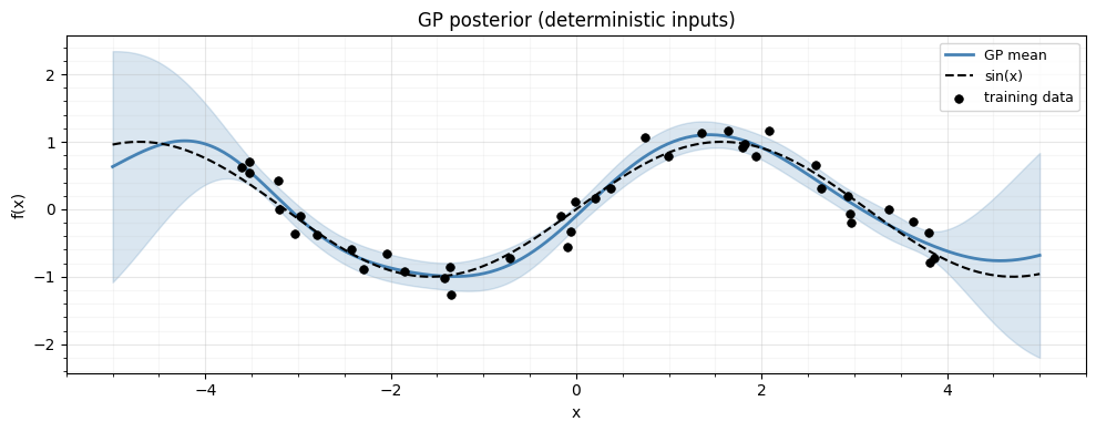

2. Single uncertain prediction¶

Now suppose our test input is uncertain: $x_* \sim \mathcal{N}(1.5, \; 0.3)$ . We compare three approaches to computing the predictive moments $\mathbb{E}[f(x_*)]$ and $\mathrm{Var}[f(x_*)]$ .

# Define the uncertain test input as a GaussianState
mu_test = jnp.array([1.5])
cov_test = lx.MatrixLinearOperator(jnp.array([[0.3]]), lx.positive_semidefinite_tag)
state_test = gaussx.GaussianState(mean=mu_test, cov=cov_test)

2a. Taylor integrator (linearisation)¶

taylor_integrator = gaussx.TaylorIntegrator()
mu_taylor, var_taylor = gaussx.uncertain_gp_predict(
    rbf_kernel, X_train, alpha, K_inv, state_test, taylor_integrator
)
print(f"Taylor:     mean = {mu_taylor:.4f},  var = {var_taylor:.4f}")

Taylor:     mean = 1.1024,  var = 0.0089

2b. Unscented integrator (sigma points)¶

unscented_integrator = gaussx.UnscentedIntegrator()
mu_ut, var_ut = gaussx.uncertain_gp_predict(
    rbf_kernel, X_train, alpha, K_inv, state_test, unscented_integrator
)
print(f"Unscented:  mean = {mu_ut:.4f},  var = {var_ut:.4f}")

Unscented:  mean = 0.9101,  var = 0.0000

2c. Monte Carlo¶

key, subkey = jr.split(key)
mu_mc, var_mc = gaussx.uncertain_gp_predict_mc(
    gp_predict_scalar, state_test, n_particles=1000, key=subkey
)
print(f"MC (1000):  mean = {mu_mc:.4f},  var = {var_mc:.4f}")

MC (1000):  mean = 0.9188,  var = 0.0724

2d. Comparison¶

All three methods should broadly agree, with Taylor slightly biased in regions of high curvature and MC showing some sampling noise.

print(f"{'Method':<14} {'Mean':>8} {'Var':>8}")
print("-" * 32)
print(f"{'Taylor':<14} {mu_taylor:8.4f} {var_taylor:8.4f}")
print(f"{'Unscented':<14} {mu_ut:8.4f} {var_ut:8.4f}")
print(f"{'MC (1000)':<14} {mu_mc:8.4f} {var_mc:8.4f}")

Method             Mean      Var
--------------------------------
Taylor           1.1024   0.0089
Unscented        0.9101   0.0000
MC (1000)        0.9188   0.0724

3. Multi-step dynamics prediction (PILCO-style)¶

This is the core idea behind PILCO: chain uncertain GP predictions to roll out a trajectory. At each step, the output distribution becomes the input for the next step, and uncertainty grows.

We use a simple 1D dynamical system: $x_{t+1} = \sin(x_t) + 0.1\,x_t + \varepsilon$ , with $\varepsilon \sim \mathcal{N}(0, 0.01)$ .

Generate dynamics data¶

dynamics_noise = 0.01

key, subkey = jr.split(key)
x_dyn = jr.uniform(subkey, (80, 1), minval=-3.0, maxval=3.0)
key, subkey = jr.split(key)
y_dyn = (
    jnp.sin(x_dyn[:, 0])
    + 0.1 * x_dyn[:, 0]
    + jnp.sqrt(dynamics_noise) * jr.normal(subkey, (80,))
)

# Train dynamics GP
K_dyn = jax.vmap(lambda x1: jax.vmap(lambda x2: rbf_kernel(x1, x2))(x_dyn))(x_dyn)
K_dyn_noisy = K_dyn + dynamics_noise * jnp.eye(x_dyn.shape[0])
K_dyn_op = lx.MatrixLinearOperator(K_dyn_noisy, lx.positive_semidefinite_tag)
alpha_dyn = gaussx.solve(K_dyn_op, y_dyn)
K_dyn_inv = lx.MatrixLinearOperator(
    jnp.linalg.inv(K_dyn_noisy), lx.positive_semidefinite_tag
)


def gp_predict_dyn(x_star):
    """Dynamics GP prediction: (D,) -> (mean, var)."""
    k_star = jax.vmap(lambda xi: rbf_kernel(x_star, xi))(x_dyn)
    mu = jnp.dot(k_star, alpha_dyn)
    solved = lx.linear_solve(K_dyn_op, k_star).value
    v = rbf_kernel(x_star, x_star) - jnp.dot(k_star, solved)
    return mu, jnp.maximum(v, 0.0)

Roll out with uncertainty propagation¶

Starting from $x_0 \sim \mathcal{N}(0.5, 0.01)$ , we chain uncertain GP predictions for $H = 15$ steps. At each step we use AssumedDensityFilter for KL-optimal Gaussian moment matching.

horizon = 15
integrator = gaussx.UnscentedIntegrator()
adf = gaussx.AssumedDensityFilter(
    n_samples=5000, regularization=1e-6, adaptive_regularization=True, key=jr.PRNGKey(0)
)

# Initial state
x0_mean = jnp.array([0.5])
x0_cov = lx.MatrixLinearOperator(jnp.array([[0.01]]), lx.positive_semidefinite_tag)
state_t = gaussx.GaussianState(mean=x0_mean, cov=x0_cov)

# Storage for trajectory
pred_means = [float(state_t.mean[0])]
pred_vars = [float(jnp.diag(state_t.cov.as_matrix())[0])]

for _t in range(horizon):
    mu_t, var_t = gaussx.uncertain_gp_predict(
        rbf_kernel, x_dyn, alpha_dyn, K_dyn_inv, state_t, integrator
    )
    # Build the next state from predicted moments
    next_mean = jnp.atleast_1d(mu_t)
    next_cov = lx.MatrixLinearOperator(
        jnp.atleast_2d(var_t + dynamics_noise), lx.positive_semidefinite_tag
    )
    state_t = gaussx.GaussianState(mean=next_mean, cov=next_cov)
    pred_means.append(float(mu_t))
    pred_vars.append(float(var_t + dynamics_noise))

pred_means = jnp.array(pred_means)
pred_stds = jnp.sqrt(jnp.array(pred_vars))

Ground truth: simulate many particles¶

n_particles = 2000
key, subkey = jr.split(key)
particles = 0.5 + jnp.sqrt(0.01) * jr.normal(subkey, (n_particles,))

true_dynamics = lambda x: jnp.sin(x) + 0.1 * x

particle_traj = [particles]
for _t in range(horizon):
    key, subkey = jr.split(key)
    noise = jr.normal(subkey, particles.shape)
    particles = true_dynamics(particles) + jnp.sqrt(dynamics_noise) * noise
    particle_traj.append(particles)

particle_means = jnp.array([p.mean() for p in particle_traj])
particle_stds = jnp.array([p.std() for p in particle_traj])

Plot: predicted trajectory vs ground truth¶

steps = jnp.arange(horizon + 1)

fig, ax = plt.subplots(figsize=(10, 4))
# Particle ground truth
ax.fill_between(
    steps,
    particle_means - 2 * particle_stds,
    particle_means + 2 * particle_stds,
    alpha=0.15,
    color="grey",
    label="MC particles (2 std)",
)
ax.plot(steps, particle_means, "k--", lw=1.5, label="MC mean", zorder=4)

# Uncertain GP rollout
ax.fill_between(
    steps,
    pred_means - 2 * pred_stds,
    pred_means + 2 * pred_stds,
    alpha=0.25,
    color="steelblue",
    label="GP rollout (2 std)",
)
ax.plot(steps, pred_means, "steelblue", lw=2, label="GP rollout mean", zorder=3)

ax.set(
    xlabel="Time step",
    ylabel="State",
    title="Multi-step uncertain GP rollout (PILCO-style)",
)
ax.legend(fontsize=9)
ax.grid(True, which="major", alpha=0.3)
ax.grid(True, which="minor", alpha=0.1)
ax.minorticks_on()
plt.tight_layout()
plt.show()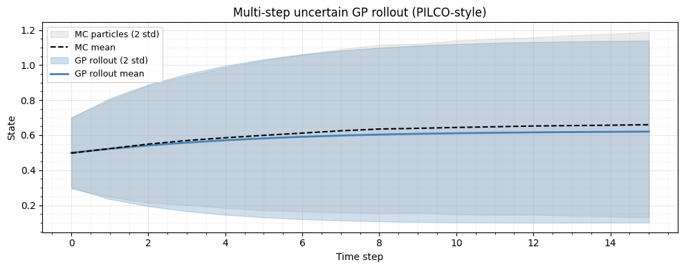

The GP rollout captures the trajectory shape while the uncertainty fans out over the horizon -- exactly the behaviour exploited by PILCO for policy gradient computation.

4. Expected cost under input uncertainty¶

In PILCO, the policy is optimised by differentiating the expected cumulative cost through the uncertain rollout. Here we compute the expected quadratic cost at a single step.

target = jnp.array([0.0])


def quadratic_cost(prediction, target):
    """Quadratic cost: (M,), (M,) -> scalar."""
    return jnp.sum((prediction - target) ** 2)


# Prediction function that maps input -> output mean
def gp_predict_mean(x):
    """GP dynamics mean prediction: (D,) -> (M,)."""
    k_star = jax.vmap(lambda xi: rbf_kernel(x, xi))(x_dyn)
    return jnp.atleast_1d(jnp.dot(k_star, alpha_dyn))


# Expected cost from an uncertain starting state
state_cost = gaussx.GaussianState(
    mean=jnp.array([1.0]),
    cov=lx.MatrixLinearOperator(jnp.array([[0.2]]), lx.positive_semidefinite_tag),
)

expected_cost = gaussx.cost_expectation(
    gp_predict_mean, quadratic_cost, state_cost, target, integrator
)
print(f"Expected quadratic cost: {expected_cost:.4f}")

Expected quadratic cost: 0.7958

This expected cost is differentiable with respect to the policy parameters (not shown here), which is the basis of PILCO’s analytic policy gradient.

5. Expectation utilities¶

gaussx provides several utilities for computing expectations under Gaussian distributions. These are the building blocks for the uncertain GP machinery above.

5a. Mean expectation: $\mathbb{E}[f(x)]$ ¶

Compute the expected value of a function under a Gaussian input.

def cubic_fn(x):
    """A simple nonlinear function: (N,) -> (N,)."""
    return x**3 - 2.0 * x


state_exp = gaussx.GaussianState(
    mean=jnp.array([1.0]),
    cov=lx.MatrixLinearOperator(jnp.array([[0.5]]), lx.positive_semidefinite_tag),
)

E_f = gaussx.mean_expectation(cubic_fn, state_exp, integrator)
print(f"E[f(x)] with Unscented: {E_f}")

# Analytic check: E[x^3 - 2x] = mu^3 + 3*mu*sigma^2 - 2*mu
mu_val, sig2_val = 1.0, 0.5
analytic = mu_val**3 + 3.0 * mu_val * sig2_val - 2.0 * mu_val
print(f"Analytic E[x^3 - 2x]:  {analytic:.4f}")

E[f(x)] with Unscented: [0.5]
Analytic E[x^3 - 2x]:  0.5000

5b. Gradient expectation: $\mathbb{E}[\nabla f(x)]$ via Stein’s lemma¶

Stein’s lemma states that for $x \sim \mathcal{N}(\mu, \Sigma)$ :

\mathbb{E}[\nabla f(x)] = \Sigma^{-1}\,\mathrm{Cov}[x, f(x)]

((3))

This is useful for computing expected gradients without differentiating through the expectation integral.

def scalar_fn(x):
    """Scalar function: (N,) -> scalar."""
    return jnp.sum(jnp.sin(x))


E_grad = gaussx.gradient_expectation(scalar_fn, state_exp, integrator)
print(f"E[nabla sin(x)] at mu=1, sigma^2=0.5: {E_grad}")

# Compare: analytic E[cos(x)] = cos(mu) * exp(-sigma^2/2)
analytic_grad = jnp.cos(1.0) * jnp.exp(-0.5 * 0.5)
print(f"Analytic E[cos(x)] (moment generating fn):  {analytic_grad:.4f}")

E[nabla sin(x)] at mu=1, sigma^2=0.5: [0.54030226]
Analytic E[cos(x)] (moment generating fn):  0.4208

5c. Log-likelihood expectation: $\mathbb{E}[\log p(y \mid f(x))]$ ¶

For variational inference and EM with uncertain inputs, we need the expected log-likelihood under the input distribution.

y_obs = 0.8


def log_likelihood_fn(x):
    """Gaussian log-likelihood: (N,) -> scalar."""
    pred = jnp.sin(x[0])
    return -0.5 * (y_obs - pred) ** 2 / noise_var - 0.5 * jnp.log(
        2.0 * jnp.pi * noise_var
    )


E_ll = gaussx.log_likelihood_expectation(log_likelihood_fn, state_exp, integrator)
print(f"E[log p(y|f(x))]: {E_ll:.4f}")

E[log p(y|f(x))]: -0.9374

6. AssumedDensityFilter with diagnostics¶

The AssumedDensityFilter projects the true (non-Gaussian) output distribution onto the closest Gaussian in KL divergence. This is the workhorse behind multi-step rollouts. The integrate_with_diagnostics method additionally returns skewness and kurtosis of the output samples, which helps assess whether the Gaussian approximation is reasonable.

6a. Well-behaved case: near-linear function¶

def mild_nonlinear(x):
    """Mildly nonlinear: (N,) -> (N,)."""
    return jnp.tanh(0.5 * x)


state_diag = gaussx.GaussianState(
    mean=jnp.array([0.0]),
    cov=lx.MatrixLinearOperator(jnp.array([[0.3]]), lx.positive_semidefinite_tag),
)

result_mild, diagnostics_mild = adf.integrate_with_diagnostics(
    mild_nonlinear, state_diag
)
print("Mild nonlinearity:")
print(f"  Predicted mean: {result_mild.state.mean}")
print(f"  Skewness:       {diagnostics_mild['skewness']}")
print(f"  Kurtosis:       {diagnostics_mild['kurtosis']}")
print("  (Gaussian: skewness ~ 0, kurtosis ~ 3)")

Mild nonlinearity:
  Predicted mean: [-0.00669525]
  Skewness:       [0.03660105]
  Kurtosis:       [2.54982357]
  (Gaussian: skewness ~ 0, kurtosis ~ 3)

6b. Challenging case: strong nonlinearity¶

def strong_nonlinear(x):
    """Highly nonlinear: (N,) -> (N,)."""
    return jnp.sin(3.0 * x) * jnp.exp(-(x**2))


state_wide = gaussx.GaussianState(
    mean=jnp.array([0.5]),
    cov=lx.MatrixLinearOperator(jnp.array([[1.0]]), lx.positive_semidefinite_tag),
)

result_strong, diagnostics_strong = adf.integrate_with_diagnostics(
    strong_nonlinear, state_wide
)
print("Strong nonlinearity:")
print(f"  Predicted mean: {result_strong.state.mean}")
print(f"  Skewness:       {diagnostics_strong['skewness']}")
print(f"  Kurtosis:       {diagnostics_strong['kurtosis']}")
print("  (Deviations from 0 / 3 indicate non-Gaussianity)")

Strong nonlinearity:
  Predicted mean: [0.0548201]
  Skewness:       [-0.05444696]
  Kurtosis:       [2.36180005]
  (Deviations from 0 / 3 indicate non-Gaussianity)

When skewness is far from zero or kurtosis far from 3, the Gaussian projection loses information. In such cases, consider:

Using more sigma points / samples
Reducing the prediction horizon
Switching to a particle-based method

Summary¶

Tool	Purpose
`uncertain_gp_predict`	Uncertain-input GP via quadrature
`uncertain_gp_predict_mc`	GP prediction with uncertain inputs via Monte Carlo
`AssumedDensityFilter`	KL-optimal Gaussian projection with diagnostics
`mean_expectation`	$\mathbb{E}[f(x)]$ under Gaussian input
`gradient_expectation`	$\mathbb{E}[\nabla f(x)]$ via Stein’s lemma
`cost_expectation`	Expected cost under input uncertainty
`log_likelihood_expectation`	$\mathbb{E}[\log p(y \mid f(x))]$

These building blocks compose naturally:

Train a GP dynamics model on observed transitions
Roll out uncertain predictions with uncertain_gp_predict
Evaluate expected cost with cost_expectation
Differentiate through the whole pipeline with jax.grad

This is the computational recipe behind PILCO and related model-based reinforcement learning algorithms.