Uncertainty Propagation through Nonlinear Functions

When a Gaussian random variable $x \sim \mathcal{N}(\mu, \Sigma)$ passes through a nonlinear function $f$ , the output $y = f(x)$ is generally not Gaussian. Different methods approximate the output distribution $p(y)$ with varying fidelity.

Motivation: uncertain inputs in Gaussian processes¶

The problem of propagating uncertainty through nonlinear maps arises naturally in Gaussian process (GP) models with uncertain inputs. At test time the input $x_*$ may itself be uncertain — for example:

In multi-step-ahead prediction with GP dynamics models (Girard et al., 2003; Deisenroth & Rasmussen, 2011), the predicted state at time $t$ becomes the uncertain input at time $t{+}1$ .
In GP-based policy search (PILCO; Deisenroth & Rasmussen, 2011), the controller must evaluate a GP whose input is a belief state.
In heteroscedastic and input-noise models (McHutchon & Rasmussen, 2011), observation noise in the inputs induces effective output noise that depends on the local gradient of the GP posterior mean.

Given a GP posterior $f \mid \mathcal{D}$ and an input distribution $x_* \sim \mathcal{N}(\mu_*, \Sigma_*)$ , we seek the predictive moments

\mathbb{E}[f(x_*)] = \int f(x)\,\mathcal{N}(x \mid \mu_*, \Sigma_*)\,dx,

((1))

\operatorname{Var}[f(x_*)] = \int \bigl(f(x) - \mathbb{E}[f(x_*)]\bigr)^2 \,\mathcal{N}(x \mid \mu_*, \Sigma_*)\,dx.

((2))

For the squared-exponential kernel these integrals have analytic forms (Quinonero-Candela et al., 2003), but for general kernels or composed models they are intractable — and the methods compared below become essential.

Methods compared¶

This notebook compares six approaches available in gaussx:

Method	Points	Key idea
Taylor 1st	1 (mean only)	Linearize $f$ at the mean
Taylor 2nd	1 + Hessian	Add curvature correction (mean only)
Taylor 2nd (var)	1 + Hessian	Curvature correction (mean + variance)
Unscented	$2N+1$ sigma points	Deterministic quadrature
Monte Carlo	$S$ random samples	Empirical moments
Pure MC	$S$ random samples	Direct histogram (ground truth)

We propagate a 1-D Gaussian through a deliberately wiggly function to expose how each method handles nonlinearity.

from __future__ import annotations

import warnings


warnings.filterwarnings("ignore", message=r".*IProgress.*")

import jax
import jax.numpy as jnp
import jax.random as jr
import lineax as lx
import matplotlib.pyplot as plt

import gaussx


jax.config.update("jax_enable_x64", True)

The nonlinear function¶

We pick a function with an inflection point, asymmetry, and saturation -- features that challenge linearisation-based methods:

f(x) = \sin(1.5\,x) \cdot \exp(-0.15\,x^2) + 0.3\,x

((3))

def f_nonlinear(x):
    """Wiggly nonlinear scalar function."""
    return jnp.sin(1.5 * x) * jnp.exp(-0.15 * x**2) + 0.3 * x


# Vectorised for plotting
f_vec = jax.vmap(f_nonlinear)

x_grid = jnp.linspace(-5, 5, 500)
y_grid = f_vec(x_grid)

fig, ax = plt.subplots(figsize=(10, 4))
ax.plot(x_grid, y_grid, "k-", lw=2)
ax.set_xlabel("x")
ax.set_ylabel("f(x)")
ax.set_title("Nonlinear function")
ax.axhline(0, c="grey", lw=0.5)
ax.grid(True, which="major", alpha=0.3)
ax.grid(True, which="minor", alpha=0.1)
ax.minorticks_on()
plt.tight_layout()
plt.show()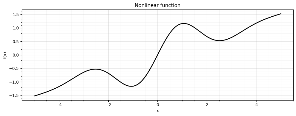

Input distribution¶

A 1-D Gaussian centred right where the function has strong curvature:

x \sim \mathcal{N}(\mu=1.0,\; \sigma^2=0.6)

((4))

mu_x = 1.0
sigma2_x = 0.6

state = gaussx.GaussianState(
    mean=jnp.array([mu_x]),
    cov=lx.MatrixLinearOperator(jnp.array([[sigma2_x]]), lx.positive_semidefinite_tag),
)

Mathematical background¶

All methods below approximate the first two moments of $y = f(x)$ when $x \sim \mathcal{N}(\mu, \Sigma)$ .

Taylor 1st order (linearisation / EKF)¶

Expand $f$ to first order around the mean:

f(x) \approx f(\mu) + J\,(x - \mu), \qquad J = \left.\frac{\partial f}{\partial x}\right|_{x=\mu}.

((5))

Under this linear approximation the output is exactly Gaussian:

\mu_y = f(\mu), \qquad \Sigma_y = J\,\Sigma\,J^\top.

((6))

This is the update used in the extended Kalman filter (EKF) (Anderson & Moore, 1979). It is exact when $f$ is affine, but ignores curvature — the mean estimate is biased whenever $f''(\mu) \neq 0$ .

Taylor 2nd order¶

Including the second-order term of the Taylor expansion gives a correction to the mean via the Hessian $H_i = \nabla^2 f_i(\mu)$ :

\mu_{y,i} = f_i(\mu) + \tfrac{1}{2}\operatorname{tr}(H_i\,\Sigma).

((7))

By default, the covariance remains the first-order expression $\Sigma_y = J\Sigma J^\top$ — this “second-order EKF” (mean-only correction) appears in Athans et al. (1968).

Optionally, with correct_variance=True, the covariance also receives a second-order correction using fourth Gaussian moments:

(\Sigma_y)_{ij} \mathrel{+}= \tfrac{1}{2}\operatorname{tr}(H_i\,\Sigma\,H_j\,\Sigma).

((8))

This can improve accuracy for mildly nonlinear functions but may overshoot for strongly nonlinear ones.

Unscented transform (UT)¶

Instead of differentiating $f$ , the UT (Julier & Uhlmann, 1997) evaluates it at a minimal set of sigma points $\{\mathcal{X}_i\}_{i=0}^{2N}$ chosen to match the mean and covariance of $x$ exactly:

\mathcal{X}_0 = \mu, \qquad \mathcal{X}_i = \mu + \bigl(\sqrt{(N+\lambda)\,\Sigma}\bigr)_i, \qquad \mathcal{X}_{N+i} = \mu - \bigl(\sqrt{(N+\lambda)\,\Sigma}\bigr)_i,

((9))

where $\lambda = \alpha^2(N + \kappa) - N$ and $(\sqrt{M})_i$ denotes the $i$ -th column of the matrix square root. The output moments are weighted sums:

\mu_y = \sum_i w_i^{(m)}\,f(\mathcal{X}_i), \qquad \Sigma_y = \sum_i w_i^{(c)}\bigl(f(\mathcal{X}_i) - \mu_y\bigr) \bigl(f(\mathcal{X}_i) - \mu_y\bigr)^\top.

((10))

The UT captures nonlinear effects up to third order for Gaussian inputs (Julier & Uhlmann, 2004) and requires no derivatives of $f$ . It underpins the unscented Kalman filter (UKF) (Wan & van der Merwe, 2000).

Monte Carlo moment matching¶

Draw $S$ samples $x^{(s)} \sim \mathcal{N}(\mu, \Sigma)$ , push them through $f$ , and compute empirical moments:

\mu_y \approx \frac{1}{S}\sum_{s=1}^S f(x^{(s)}), \qquad \Sigma_y \approx \frac{1}{S}\sum_{s=1}^S \bigl(f(x^{(s)}) - \mu_y\bigr)\bigl(f(x^{(s)}) - \mu_y\bigr)^\top.

((11))

This is unbiased and converges at rate $O(1/\sqrt{S})$ regardless of dimension — making it the method of choice when $N$ is large or $f$ is very nonlinear. The moment-matched Gaussian is the best Gaussian approximation in the KL sense and is used for “assumed density filtering” in GP dynamics models (Deisenroth & Rasmussen, 2011).

Run all six methods¶

# --- Taylor 1st order (EKF) ---
taylor1 = gaussx.TaylorIntegrator(order=1)
res_t1 = taylor1.integrate(lambda x: jnp.atleast_1d(f_nonlinear(x[0])), state)

# --- Taylor 2nd order (mean correction only, default) ---
taylor2 = gaussx.TaylorIntegrator(order=2)
res_t2 = taylor2.integrate(lambda x: jnp.atleast_1d(f_nonlinear(x[0])), state)

# --- Taylor 2nd order (mean + variance correction) ---
taylor2v = gaussx.TaylorIntegrator(order=2, correct_variance=True)
res_t2v = taylor2v.integrate(lambda x: jnp.atleast_1d(f_nonlinear(x[0])), state)

# --- Unscented transform ---
ut = gaussx.UnscentedIntegrator(alpha=1.0, beta=2.0, kappa=0.0)
res_ut = ut.integrate(lambda x: jnp.atleast_1d(f_nonlinear(x[0])), state)

# --- Monte Carlo integrator (moment matching) ---
mc = gaussx.MonteCarloIntegrator(n_samples=50_000, key=jr.key(42))
res_mc = mc.integrate(lambda x: jnp.atleast_1d(f_nonlinear(x[0])), state)

# --- Pure MC: raw histogram as ground truth ---
key = jr.key(123)
n_pure = 200_000
x_samples = mu_x + jnp.sqrt(sigma2_x) * jr.normal(key, (n_pure,))
y_samples = f_vec(x_samples)
pure_mc_mean = jnp.mean(y_samples)
pure_mc_var = jnp.var(y_samples)

def _moments(res):
    m = float(res.state.mean[0])
    v = float(res.state.cov.as_matrix()[0, 0])
    return m, v


methods = {
    "Taylor 1st": _moments(res_t1),
    "Taylor 2nd": _moments(res_t2),
    "Taylor 2nd (var)": _moments(res_t2v),
    "Unscented": _moments(res_ut),
    "MC (50k)": _moments(res_mc),
    "Pure MC (200k)": (float(pure_mc_mean), float(pure_mc_var)),
}

print(f"{'Method':<18s} {'Mean':>8s} {'Std':>8s}")
print("-" * 36)
for name, (m, v) in methods.items():
    print(f"{name:<18s} {m:8.4f} {jnp.sqrt(v):8.4f}")

Method                 Mean      Std
------------------------------------
Taylor 1st           1.1586   0.1036
Taylor 2nd           0.5085   0.1036
Taylor 2nd (var)     0.5085   0.9251
Unscented            0.6085   0.8062
MC (50k)             0.7388   0.5023
Pure MC (200k)       0.7358   0.5074

Visualisation¶

The main plot shows:

Bottom x-axis: the input Gaussian $p(x)$ as a filled curve.
Left y-axis: the nonlinear function $f(x)$ (black curve).
Right side: the output Gaussian approximations from each method, and the true output histogram from pure MC.

This makes it easy to see how the input bell curve “warps” through $f$ and how each approximation captures (or misses) the resulting skew.

from matplotlib.patches import FancyArrowPatch
from scipy.stats import norm


fig, ax = plt.subplots(figsize=(9, 6))

# --- Nonlinear function (clip to x < x_right so it doesn't bleed) ---
x_fn = jnp.linspace(-4, 3.5, 400)
y_fn = f_vec(x_fn)
ax.plot(x_fn, y_fn, "k-", lw=2.5, label="$f(x)$", zorder=5)

# --- Input Gaussian (along x-axis) ---
x_pdf = norm.pdf(x_grid, loc=mu_x, scale=jnp.sqrt(sigma2_x))
# Scale so the peak is visually ~0.8 units tall on the y-axis
x_pdf_scaled = x_pdf / x_pdf.max() * 0.8
y_base = -2.0  # shift below the function
ax.fill_between(
    x_grid,
    y_base,
    y_base + x_pdf_scaled,
    color="C0",
    alpha=0.3,
    zorder=2,
)
ax.plot(x_grid, y_base + x_pdf_scaled, "C0-", lw=1.5, zorder=3)
ax.text(
    mu_x,
    y_base - 0.15,
    r"$p(x)$",
    ha="center",
    fontsize=12,
    color="C0",
)

# --- Output distributions (horizontal Gaussians) ---
colours = ["C1", "C2", "C6", "C3", "C4", "C5"]
x_right = 4.2
width = 1.0

y_range = jnp.linspace(-2.5, 3.0, 400)

for i, (name, (m, v)) in enumerate(methods.items()):
    s = jnp.sqrt(v)
    pdf_vals = norm.pdf(y_range, loc=m, scale=s)
    pdf_scaled = pdf_vals / pdf_vals.max() * width
    x_pos = x_right + i * 0.9

    ax.fill_betweenx(
        y_range,
        x_pos,
        x_pos + pdf_scaled,
        color=colours[i],
        alpha=0.35,
        zorder=2,
    )
    ax.plot(
        x_pos + pdf_scaled,
        y_range,
        color=colours[i],
        lw=1.5,
        zorder=3,
    )
    ax.plot(x_pos, m, "o", color=colours[i], ms=5, zorder=6)
    ax.text(
        x_pos + width * 0.5,
        3.3,
        name,
        ha="center",
        fontsize=8,
        color=colours[i],
        rotation=45,
        fontweight="bold",
    )

# --- Pure MC histogram (faint, behind the Gaussians) ---
hist_x_pos = x_right + 5 * 0.9
counts, bin_edges = jnp.histogram(y_samples, bins=80, density=True)
bin_centres = 0.5 * (bin_edges[:-1] + bin_edges[1:])
hist_scaled = counts / counts.max() * width
ax.barh(
    bin_centres,
    hist_scaled,
    left=hist_x_pos,
    height=bin_edges[1] - bin_edges[0],
    color="C5",
    alpha=0.2,
    zorder=1,
)

# --- Arrow showing the "propagation" ---
arrow = FancyArrowPatch(
    (mu_x, f_nonlinear(jnp.array(mu_x))),
    (x_right - 0.3, float(res_ut.state.mean[0])),
    arrowstyle="-|>",
    color="grey",
    lw=1.5,
    connectionstyle="arc3,rad=0.2",
    zorder=4,
)
ax.add_patch(arrow)
ax.text(
    (mu_x + x_right - 0.3) / 2,
    float(res_ut.state.mean[0]) + 0.5,
    "propagate\nuncertainty",
    ha="center",
    fontsize=9,
    color="grey",
)

# --- Formatting ---
ax.set_xlim(-4, x_right + 6 * 0.9 + 1.5)
ax.set_ylim(y_base - 0.4, 4.0)
ax.set_xlabel("x", fontsize=12)
ax.set_ylabel("y = f(x)", fontsize=12)
ax.set_title(
    r"Uncertainty propagation: input $\to$ nonlinear $f$ $\to$ output",
    fontsize=13,
)
ax.axhline(0, c="grey", lw=0.4)
ax.legend(loc="upper left", fontsize=9)
ax.grid(True, which="major", alpha=0.3)
ax.grid(True, which="minor", alpha=0.1)
ax.minorticks_on()
plt.tight_layout()
plt.show()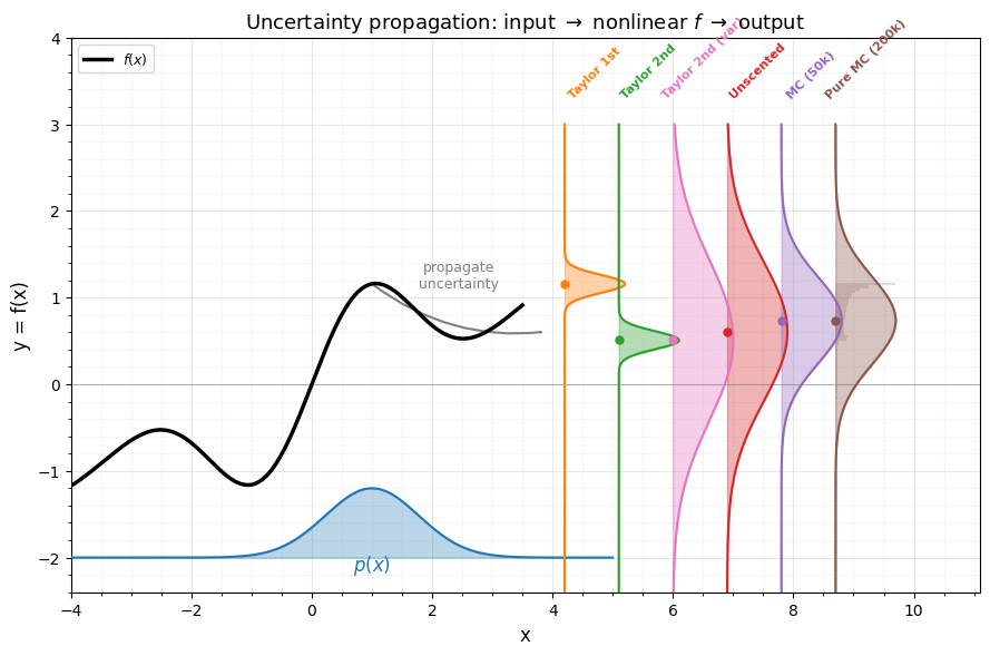

Observations¶

Taylor 1st order uses only the local slope at μ -- it produces a symmetric Gaussian whose width depends on $|f'(\mu)|$ . When $f$ curves strongly, this misses the mean shift.
Taylor 2nd order adds a Hessian correction to the mean ( $\mu_y \mathrel{+}= \tfrac{1}{2}\operatorname{tr}(H \Sigma)$ ) and gets closer to the true mean, but the covariance is still first-order.
Taylor 2nd (var) additionally corrects the covariance using fourth Gaussian moments. For this wiggly function the correction overshoots — a common failure mode for strongly nonlinear functions.
Unscented transform evaluates $f$ at $2N{+}1=3$ deterministic sigma points and captures the nonlinearity much better -- even with just 3 function evaluations.
Monte Carlo (moment matching) converges to the true moments with enough samples. With 50k samples, the mean and variance match the pure MC histogram closely.
The pure MC histogram reveals that the true output distribution is slightly skewed -- something no Gaussian approximation can capture. All four methods project onto the best-fit Gaussian, which is the optimal thing to do for downstream linear-Gaussian inference (Kalman updates, variational inference, etc.).

Error comparison¶

ref_mean, ref_var = float(pure_mc_mean), float(pure_mc_var)

fig, axes = plt.subplots(1, 2, figsize=(10, 3.5))

names = list(methods.keys())[:-1]
mean_errors = [abs(methods[n][0] - ref_mean) for n in names]
var_errors = [abs(methods[n][1] - ref_var) for n in names]
colours_bar = colours[:5]

axes[0].bar(
    names,
    mean_errors,
    color=colours_bar,
    alpha=0.7,
    edgecolor="k",
    lw=0.5,
)
axes[0].set_ylabel("|mean error|")
axes[0].set_title("Mean error vs. pure MC reference")
axes[0].tick_params(axis="x", rotation=25)
axes[0].grid(True, which="major", alpha=0.3)
axes[0].grid(True, which="minor", alpha=0.1)
axes[0].minorticks_on()

axes[1].bar(
    names,
    var_errors,
    color=colours_bar,
    alpha=0.7,
    edgecolor="k",
    lw=0.5,
)
axes[1].set_ylabel("|variance error|")
axes[1].set_title("Variance error vs. pure MC reference")
axes[1].tick_params(axis="x", rotation=25)
axes[1].grid(True, which="major", alpha=0.3)
axes[1].grid(True, which="minor", alpha=0.1)
axes[1].minorticks_on()

plt.tight_layout()
plt.show()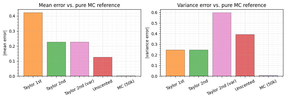

When to use each method¶

Method	Cost	Best for
Taylor 1st	$O(N^2)$ Jacobian	Mildly nonlinear, real-time EKF
Taylor 2nd	$O(N^3)$ Hessian	Moderate nonlinearity, small $N$
Unscented	$O(N)$ function evals	Good default; no derivatives needed
Monte Carlo	$O(S)$ function evals	Complex functions, large $N$ , reference

All four methods are available in gaussx via the AbstractIntegrator interface, so you can swap them with a single line change:

integrator = gaussx.TaylorIntegrator(order=1)    # or
integrator = gaussx.UnscentedIntegrator()         # or
integrator = gaussx.MonteCarloIntegrator(n_samples=10000, key=jr.key(0))

result = integrator.integrate(f, state)

Connection to GP prediction with uncertain inputs¶

In a trained GP with posterior mean $m(x)$ and variance $v(x)$ , the total predictive variance under input uncertainty decomposes as (Girard et al., 2003, Eq. 2.40):

\operatorname{Var}[y_*] \;=\; \underbrace{\mathbb{E}_{x_*}[v(x_*)]}_{\text{noise / model variance}} \;+\; \underbrace{\operatorname{Var}_{x_*}[m(x_*)]}_{\text{input uncertainty}}.

((12))

The first term averages the GP’s own uncertainty over plausible inputs; the second is exactly the output variance computed by the methods above, applied to the posterior mean function $m$ .

For the squared-exponential (RBF) kernel, both expectations can be evaluated in closed form because the required Gaussian-times-kernel integrals are themselves Gaussian (Quinonero-Candela et al., 2003; Deisenroth, 2010, Appendix A). For other kernels (Matern, periodic, neural-network, etc.) or for compositions of GPs (deep GPs), the integrals are intractable and the numerical methods in this notebook are the standard approach.

The PILCO algorithm (Deisenroth & Rasmussen, 2011) chains these moment-matching steps across a planning horizon $T$ to perform gradient-based policy search in continuous state spaces, using the analytic RBF moments where possible and falling back to the unscented transform for the policy mapping.

References¶

Anderson, B. D. O. & Moore, J. B. (1979). Optimal Filtering. Prentice-Hall.
Athans, M., Wishner, R. P., & Bertolini, A. (1968). Suboptimal state estimation for continuous-time nonlinear systems from discrete noisy measurements. IEEE Trans. Automatic Control, 13(5), 504--514.
Deisenroth, M. P. (2010). Efficient Reinforcement Learning using Gaussian Processes. PhD thesis, Karlsruhe Institute of Technology.
Deisenroth, M. P. & Rasmussen, C. E. (2011). PILCO: A model-based and data-efficient approach to policy search. Proc. ICML, 465--472.
Girard, A., Rasmussen, C. E., Quinonero-Candela, J., & Murray-Smith, R. (2003). Gaussian process priors with uncertain inputs — application to multiple-step ahead time series forecasting. Proc. NeurIPS 15.
Julier, S. J. & Uhlmann, J. K. (1997). A new extension of the Kalman filter to nonlinear systems. Proc. AeroSense, 182--193.
Julier, S. J. & Uhlmann, J. K. (2004). Unscented filtering and nonlinear estimation. Proc. IEEE, 92(3), 401--422.
McHutchon, A. & Rasmussen, C. E. (2011). Gaussian process training with input noise. Proc. NeurIPS 24.
Quinonero-Candela, J., Girard, A., Larsen, J., & Rasmussen, C. E. (2003). Propagation of uncertainty in Bayesian kernel models — application to multiple-step ahead forecasting. Proc. ICASSP.
Wan, E. A. & van der Merwe, R. (2000). The unscented Kalman filter for nonlinear estimation. Proc. IEEE Adaptive Systems for Signal Processing, Communications, and Control Symposium, 153--158.