Double Gyre — Barotropic QG - somax: Simple Ocean Models in JAX

The wind-driven double gyre is the canonical wind-forced ocean-basin test: a sinusoidal wind-stress curl spins up two counter-rotating gyres, the $\beta$ -effect concentrates the return flow into a narrow western boundary current, and — at low enough viscosity — that current goes barotropically unstable into a meandering eastward jet that sheds eddies (geostrophic turbulence).

Barotropic quasi-geostrophic is the cheapest model that captures it: a single potential-vorticity field, advected by the energy- and enstrophy-conserving Arakawa Jacobian and inverted to a streamfunction with a spectral Poisson solve. The enstrophy-conserving advection is what lets the run stay stable in the turbulent (eddy-permitting) regime even though the grid-Reynolds number is well above the centred-advection limit.

This page executes a 64² turbulent run (cheap, ~minutes) and then gives ready-to-run, correctly-scaled commands for 128²–1024² that you can launch in your own time (256²+ wants a GPU). It follows the repo’s getting-sims-to-work methodology throughout: observability first, probe cost before committing, and scale forcing/viscosity/dt with the resolution.

import time

import diffrax as dfx
import jax
import jax.numpy as jnp
import matplotlib.pyplot as plt
import numpy as np
from finitevolx import Difference2D

from somax.models import BarotropicQG, BarotropicQGState

# Fixed physics for the whole resolution sweep: a 1000 km square basin, a
# mid-latitude beta-plane, a double-gyre wind, and linear bottom drag. Only the
# numerics (viscosity and dt) change with resolution.
LX = LY = 1.0e6
F0, BETA = 1.0e-4, 1.6e-11
WIND = 2.0e-11  # wind-stress-curl amplitude (turbulent regime)
DRAG = 1.0e-7  # linear bottom drag (1/s)
NU0_AT_64 = 150.0  # lateral viscosity at 64^2; scaled down with dx below


def build_model(nx: int) -> BarotropicQG:
    """Barotropic-QG double gyre at resolution ``nx`` with resolution-scaled ν.

    The physics (domain, beta, wind, drag) is fixed; the lateral viscosity is
    scaled **linearly with the grid spacing**, ``ν = 150·(64/nx)``, so the
    grid-Reynolds number stays in the same eddy-resolving band as resolution
    increases (finer grids resolve smaller eddies, so they need — and tolerate —
    less viscosity). At every resolution this stays at/below the Munk-layer
    viscosity, i.e. deliberately eddy-permitting.
    """
    nu = NU0_AT_64 * (64.0 / nx)
    return BarotropicQG.create(
        nx=nx,
        ny=nx,
        Lx=LX,
        Ly=LY,
        f0=F0,
        beta=BETA,
        lateral_viscosity=nu,
        bottom_drag=DRAG,
        wind_amplitude=WIND,
        wind_profile="doublegyre",
    )


def recommended_dt(nx: int) -> float:
    """Starting `dt` (s), scaled from the 64² value by the advective CFL.

    The jet speed grows as the grid sharpens, so `dt` must shrink. `dt ∝ dx`
    (``600·(64/nx)``) is a safe first guess; confirm it with :func:`probe`,
    which reports ``|u|_max`` and the implied CFL-limited `dt`.
    """
    return 600.0 * (64.0 / nx)

Observability + start-small helpers¶

probe runs a short window and reports the two numbers that decide whether a long run is worth launching: ms/step (so you can extrapolate the cost) and |u|_max (so you can check the advective CFL dt < dx/|u|). run does the full integration, checks finiteness, and saves the arrays to disk before any plotting so a plotting bug can never waste the integration.

def probe(nx: int, days: float = 180.0) -> None:
    """Short smoke + cost/CFL probe — run this BEFORE any long integration."""
    model = build_model(nx)
    s0 = BarotropicQGState(q=jnp.zeros((model.grid.Ny, model.grid.Nx)))
    dt = recommended_dt(nx)
    t1 = days * 86400.0
    t = time.time()
    sol = model.integrate(
        s0,
        t0=0.0,
        t1=t1,
        dt=dt,
        saveat=dfx.SaveAt(ts=jnp.array([t1])),
        max_steps=20_000_000,
    )
    jax.block_until_ready(sol.ys.q)
    el = time.time() - t
    n = int(t1 / dt)
    psi = np.asarray(model._invert_pv(sol.ys.q[-1]))[2:-2, 2:-2]
    u = -np.gradient(psi, model.grid.dy, axis=0)
    v = np.gradient(psi, model.grid.dx, axis=1)
    umax = float(np.sqrt(u**2 + v**2).max())
    finite = bool(jnp.all(jnp.isfinite(sol.ys.q)))
    print(
        f"{nx:>4}²  dx={model.grid.dx / 1e3:5.1f} km  ν={model.params.lateral_viscosity:6.1f}"
        f"  dt={dt:6.0f}s  {el / n * 1e3:6.2f} ms/step  finite={finite}"
        f"  |u|max={umax:5.2f} m/s  CFL-dt≈{0.4 * model.grid.dx / max(umax, 1e-6):5.0f}s"
    )


def run(nx: int, years: float, dt: float | None = None, save: str | None = None):
    """Full spin-up; finiteness-checked; arrays saved before plotting."""
    model = build_model(nx)
    s0 = BarotropicQGState(q=jnp.zeros((model.grid.Ny, model.grid.Nx)))
    dt = recommended_dt(nx) if dt is None else dt
    t1 = years * 31557600.0
    sol = model.integrate(
        s0,
        t0=0.0,
        t1=t1,
        dt=dt,
        saveat=dfx.SaveAt(ts=jnp.array([t1])),
        max_steps=50_000_000,
    )
    jax.block_until_ready(sol.ys.q)
    q = sol.ys.q[-1]
    assert bool(jnp.all(jnp.isfinite(q))), "non-finite — drop dt or raise ν"
    diff = Difference2D(grid=model.grid)
    psi_f = np.asarray(model._invert_pv(q))
    zeta_f = np.asarray(
        diff.curl(
            -diff.diff_y_T_to_V(jnp.asarray(psi_f)),
            diff.diff_x_T_to_U(jnp.asarray(psi_f)),
        )
    )
    psi = psi_f[2:-2, 2:-2]
    zeta = zeta_f[2:-2, 2:-2]
    u = -np.gradient(psi, model.grid.dy, axis=0)
    v = np.gradient(psi, model.grid.dx, axis=1)
    ke = 0.5 * (u**2 + v**2)
    x = np.asarray(jnp.arange(model.grid.Nx) * model.grid.dx)[2:-2] / 1e3
    y = np.asarray(jnp.arange(model.grid.Ny) * model.grid.dy)[2:-2] / 1e3
    if save is not None:  # checkpoint BEFORE plotting
        np.savez(save, psi=psi, ke=ke, zeta=zeta, x=x, y=y)
    diag = model.diagnose(BarotropicQGState(q=q))
    print(
        f"{nx}²  {years:g} yr  KE={float(diag.kinetic_energy):.3e}"
        f"  enstrophy={float(diag.enstrophy):.3e}  |u|max={float(np.sqrt(u**2 + v**2).max()):.2f} m/s"
    )
    return x, y, psi, ke, zeta

Executed run — 64², turbulent (3 yr)¶

Low viscosity (ν=150) and a moderate wind (2e-11) put this in the eddy-permitting regime; the boundary current destabilises into a meandering jet within the first year or two.

x, y, psi, ke, zeta = run(nx=64, years=3.0, dt=600.0)

64²  3 yr  KE=1.601e+13  enstrophy=7.932e+02  |u|max=10.57 m/s

Streamfunction, kinetic energy, and the eddy field¶

$\psi$ (the gyres + boundary current), kinetic energy $\tfrac{1}{2}(u^2+v^2)$ (lights up the jet and eddies), and relative vorticity $\zeta$ (the clearest view of the turbulent eddy field).

fig, axes = plt.subplots(1, 3, figsize=(17, 5.2))
mp = np.percentile(np.abs(psi), 99.5) or 1.0
c0 = axes[0].contourf(x, y, psi, levels=23, cmap="RdBu_r", vmin=-mp, vmax=mp)
axes[0].set_title("Streamfunction  ψ")
plt.colorbar(c0, ax=axes[0], label="m²/s")
c1 = axes[1].contourf(
    x, y, ke, levels=23, cmap="inferno", vmin=0.0, vmax=np.percentile(ke, 99.5) or 1.0
)
axes[1].set_title("Kinetic energy  ½(u²+v²)")
plt.colorbar(c1, ax=axes[1], label="m²/s²")
mz = np.percentile(np.abs(zeta), 99.0) or 1.0
c2 = axes[2].contourf(x, y, zeta, levels=23, cmap="RdBu_r", vmin=-mz, vmax=mz)
axes[2].set_title("Relative vorticity  ζ")
plt.colorbar(c2, ax=axes[2], label="1/s")
for ax in axes:
    ax.set_xlabel("x (km)")
    ax.set_ylabel("y (km)")
    ax.set_aspect("equal")
fig.suptitle("Barotropic QG double gyre — 64², turbulent, 3 yr", y=1.03)
plt.tight_layout()
plt.show()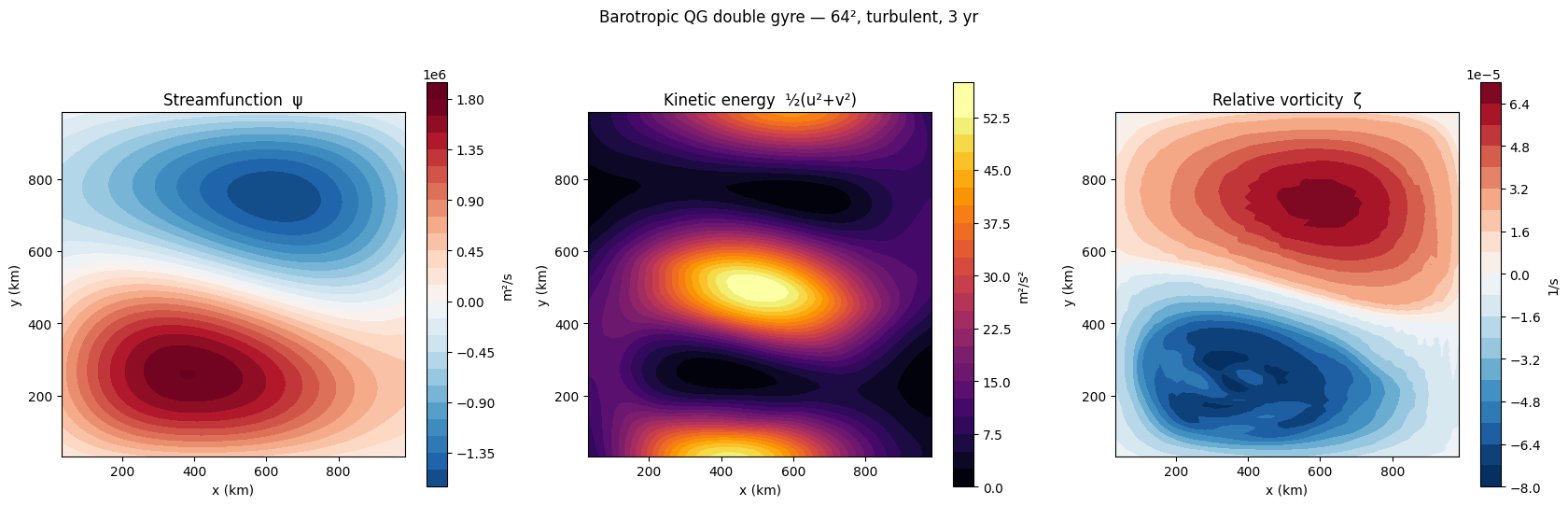

Scaling up — 128², 256², 512², 1024² (run in your spare time)¶

The helpers above already encode the scaling, so a higher-resolution sweep is a one-liner. Always probe first, then launch the full run. The finer the grid the more of the turbulent cascade you resolve (sharper jet, more eddies, filaments) — and the more it costs.

nx	dx	ν (=150·64/nx)	dt (start)	rough cost, 10 yr, CPU*
64	15.6 km	150	600 s	minutes
128	7.8 km	75	300 s	~1 hr
256	3.9 km	37.5	150 s	~8 hr (use a GPU)
512	2.0 km	18.75	75 s	days (GPU)
1024	1.0 km	9.375	37.5 s	~1 week (GPU)

*Cost grows roughly as nx³ (the grid is nx² and dt ∝ 1/nx); a GPU is strongly recommended at 256² and above. JAX runs the same code on GPU unchanged — just install a CUDA jaxlib.

# 1) Probe every resolution first (ms/step, |u|max, CFL-limited dt):
for nx in (128, 256, 512, 1024):
    probe(nx)

# 2) Launch a full turbulent spin-up at the resolution you want, checkpointing
#    the fields to disk (re-plot from the .npz, never re-integrate):
x, y, psi, ke, zeta = run(nx=256, years=10.0, save="dg_bt_256.npz")

# If probe() reports the suggested CFL-dt is below recommended_dt(nx), pass it
# explicitly, e.g. run(nx=256, years=10.0, dt=120.0, save="dg_bt_256.npz").

Then plot from the saved arrays with the same three-panel code as above:

d = np.load("dg_bt_256.npz")
x, y, psi, ke, zeta = d["x"], d["y"], d["psi"], d["ke"], d["zeta"]
# ... same contourf panels ...

Notes¶

Resolution ↔ forcing ↔ viscosity ↔ dt are coupled. Here the physics (wind, drag, domain, β) is held fixed and only ν and dt scale with the grid: ν shrinks ∝ dx to stay eddy-resolving, and dt shrinks because the sharper jet tightens the advective CFL dt < dx/|u|.
QG removes the external gravity-wave CFL (no √(gH) term), so dt is set by advection, not waves.
Stability in this high-grid-Reynolds regime comes from the enstrophy-conserving Arakawa Jacobian + bottom drag, not from viscosity.
See the getting-sims-to-work skill for the full bring-up checklist.