Step 1 — 1D Linear Convection - somax: Simple Ocean Models in JAX

13 Steps to Navier-Stokes with somax (inspired by Lorena Barba’s CFD Python)

The linear convection equation is the simplest PDE in computational fluid dynamics. It describes how a disturbance propagates through a medium at a constant speed without changing shape (in the continuous limit). Mastering this equation gives you the foundation for every subsequent step.

What you’ll learn:

The physics of linear wave propagation and the CFL condition
How to set up a 1D PDE model in somax
How to compare numerical output against the analytical solution
How to differentiate through the simulation with eqx.filter_grad

The PDE¶

\frac{\partial u}{\partial t} + c \frac{\partial u}{\partial x} = 0

(1)

where $c$ is the constant wave speed. The exact solution for an initial condition $u(x, 0) = u_0(x)$ is simply:

u(x, t) = u_0(x - ct)

(2)

The initial profile translates to the right at speed $c$ without distortion. This is pure advection — no diffusion, no steepening.

The CFL condition¶

The Courant-Friedrichs-Lewy (CFL) number $\nu_{\mathrm{CFL}} = c \, \Delta t / \Delta x$ must satisfy $\nu_{\mathrm{CFL}} \le 1$ for explicit upwind schemes. If the numerical domain of dependence does not contain the physical domain of dependence, the scheme is unstable.

Grid layout and boundary conditions¶

somax uses the Arakawa C-grid from finitevolX. In 1D, scalar fields (like $u$ ) live at T-points (cell centres) and fluxes are computed at U-points (cell edges):

 ghost                    interior                     ghost
 ┌─────┬──────┬──────┬──────┬──────┬──────┬──────┬─────┐
 │  G  │  T₁  │  T₂  │  T₃  │ ···  │ Tₙ₋₁│  Tₙ  │  G  │
 └──┬──┴──┬───┴──┬───┴──┬───┴──┬───┴──┬───┴──┬───┴──┬──┘
    U₀    U₁     U₂     U₃           Uₙ₋₁    Uₙ    Uₙ₊₁
         ←── dx ──→

T-points (indices 1:-1): where u is stored and updated
U-points: where Difference1D computes derivatives
Ghost cells (indices 0 and -1): filled by BCs before each RHS evaluation

Periodic BCs copy the last interior value into the opposite ghost cell:

 u[0] = u[-2]      (left ghost ← rightmost interior)
 u[-1] = u[1]      (right ghost ← leftmost interior)

This makes the domain wrap around so waves that exit one side re-enter from the other.

from __future__ import annotations

import diffrax as dfx
import equinox as eqx
import jax
import jax.numpy as jnp
import matplotlib.pyplot as plt

from somax.models import LinearConvection1D, LinearConvection1DState

1. Create the model¶

LinearConvection1D.create() builds a model on a 1D Arakawa C-grid with nx interior cells spanning a domain of length Lx. The wave speed c is a differentiable parameter visible to jax.grad.

nx, Lx, c = 200, 4.0, 1.0
model = LinearConvection1D.create(nx=nx, Lx=Lx, c=c)

print(f"Grid: Nx={model.grid.Nx} (includes 2 ghost cells), dx={model.grid.dx:.4f}")
print(f"Wave speed c = {float(model.params.c):.1f}")

Grid: Nx=202 (includes 2 ghost cells), dx=0.0200
Wave speed c = 1.0

2. Initial condition¶

We use a Gaussian bump centered at $x = 1.0$ with standard deviation $\sigma = 0.2$ . The state array has shape (Nx,) which includes the two ghost cells that enforce periodic boundary conditions.

x = jnp.arange(model.grid.Nx) * model.grid.dx

mu0, sigma0 = 1.0, 0.2
u0 = jnp.exp(-0.5 * ((x - mu0) / sigma0) ** 2)

state0 = LinearConvection1DState(u=u0)

fig, ax = plt.subplots(figsize=(8, 3))
ax.plot(x[1:-1], u0[1:-1], color="steelblue", lw=1.5, label="u(x, 0)")
ax.set_xlabel("x")
ax.set_ylabel("u")
ax.set_title("Initial condition: Gaussian bump")
ax.legend()
ax.grid(True, alpha=0.3)
plt.tight_layout()
plt.show()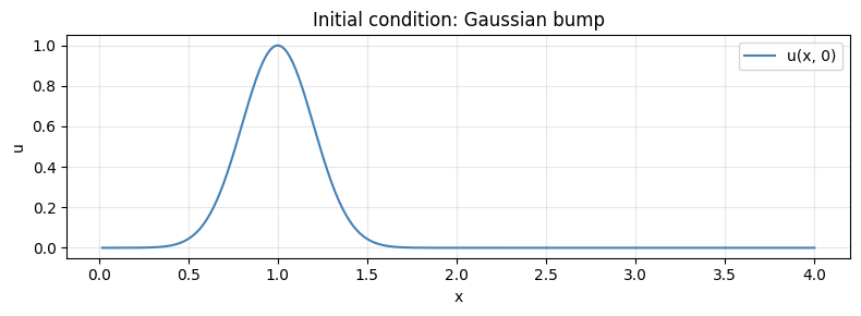

3. Forward simulation¶

We integrate from $t = 0$ to $t = 0.5$ using model.integrate(). The method wraps diffrax.diffeqsolve and automatically applies periodic boundary conditions at every RHS evaluation.

t0, t1, dt = 0.0, 0.5, 0.002
ts = jnp.linspace(t0, t1, 6)  # save at 6 snapshots

sol = model.integrate(
    state0,
    t0=t0,
    t1=t1,
    dt=dt,
    saveat=dfx.SaveAt(ts=ts),
)

print(f"Trajectory shape: u={sol.ys.u.shape}")
print(f"CFL number: c * dt / dx = {c * dt / model.grid.dx:.3f}")

Trajectory shape: u=(6, 202)
CFL number: c * dt / dx = 0.100

4. Visualize the wave propagation¶

The Gaussian translates to the right at speed $c = 1$ . After $t = 0.5$ it should have moved by $\Delta x = 0.5$ .

colors_snap = ["#2196F3", "#4CAF50", "#FF9800", "#9C27B0", "#F44336", "#795548"]

fig, ax = plt.subplots(figsize=(10, 4))
for i, t_snap in enumerate(ts):
    ax.plot(
        x[1:-1],
        sol.ys.u[i, 1:-1],
        color=colors_snap[i],
        lw=1.5,
        label=f"t = {float(t_snap):.2f}",
    )
ax.set_xlabel("x")
ax.set_ylabel("u")
ax.set_title("1D Linear Convection — Wave Propagation")
ax.legend(fontsize=9, ncol=2)
ax.grid(True, alpha=0.3)
plt.tight_layout()
plt.show()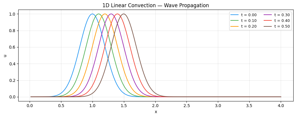

5. Comparison with the analytical solution¶

The exact solution is $u(x, t) = u_0(x - ct)$ . With periodic BCs the shifted coordinate wraps around the domain.

u_final_numerical = sol.ys.u[-1]
x_shifted = (x - c * float(ts[-1])) % Lx
u_exact = jnp.exp(-0.5 * ((x_shifted - mu0) / sigma0) ** 2)

fig, axes = plt.subplots(1, 2, figsize=(12, 4))

# Overlay
ax = axes[0]
ax.plot(x[1:-1], u_exact[1:-1], "k--", lw=1.5, label="Analytical")
ax.plot(x[1:-1], u_final_numerical[1:-1], color="steelblue", lw=1.5, label="Numerical")
ax.set_xlabel("x")
ax.set_ylabel("u")
ax.set_title(f"Profile at t = {float(ts[-1]):.2f}")
ax.legend()
ax.grid(True, alpha=0.3)

# Error
ax = axes[1]
error = jnp.abs(u_final_numerical - u_exact)
ax.plot(x[1:-1], error[1:-1], color="crimson", lw=1.0)
ax.set_xlabel("x")
ax.set_ylabel("|error|")
ax.set_title("Pointwise absolute error")
ax.grid(True, alpha=0.3)

plt.tight_layout()
plt.show()

print(f"Max error: {float(jnp.max(error[1:-1])):.6f}")
print(f"L2 error:  {float(jnp.sqrt(jnp.sum(error[1:-1] ** 2) * model.grid.dx)):.6f}")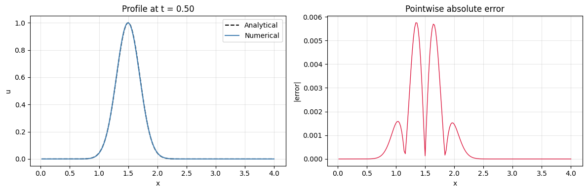

Max error: 0.005749
L2 error:  0.003391

6. Diagnostics — energy conservation¶

For the linear convection equation with periodic BCs, the total energy $E = \frac{1}{2} \int u^2 \, dx$ is conserved analytically. Numerical dissipation causes a slow decay.

ts_dense = jnp.linspace(t0, t1, 100)
sol_dense = model.integrate(
    state0,
    t0=t0,
    t1=t1,
    dt=dt,
    saveat=dfx.SaveAt(ts=ts_dense),
)

energy = jax.vmap(model.diagnose)(sol_dense.ys).energy

fig, ax = plt.subplots(figsize=(8, 3))
ax.plot(ts_dense, energy, color="teal", lw=1.5)
ax.set_xlabel("Time")
ax.set_ylabel("Energy")
ax.set_title("Energy over time (should be approximately conserved)")
ax.grid(True, alpha=0.3)
plt.tight_layout()
plt.show()

print(f"Energy: initial = {float(energy[0]):.6f}, final = {float(energy[-1]):.6f}")
print(f"Relative change: {abs(float(energy[-1] - energy[0])) / float(energy[0]):.4%}")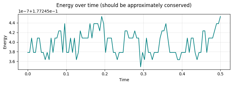

Energy: initial = 0.177245, final = 0.177245
Relative change: 0.0000%

7. Differentiability demo¶

One of the key advantages of somax is that every simulation is end-to-end differentiable. We define a loss function and compute $\partial \mathcal{L} / \partial c$ — the gradient of the loss with respect to the wave speed parameter.

# Target: we want the final profile to match a Gaussian at x=1.5
x_target = 1.5
u_target = jnp.exp(-0.5 * ((x - x_target) / sigma0) ** 2)


@eqx.filter_grad
def grad_wrt_model(m):
    """Gradient of MSE loss w.r.t. all differentiable model parameters."""
    sol = m.integrate(state0, t0=0.0, t1=0.5, dt=0.002)
    u_pred = sol.ys.u[-1]
    return jnp.mean((u_pred[1:-1] - u_target[1:-1]) ** 2)


grads = grad_wrt_model(model)

print("--- Gradient w.r.t. model parameters ---")
print(f"  dL/d(c) = {float(grads.params.c):.6f}")
print()
print("The gradient tells us how to adjust the wave speed to move")
print("the final profile closer to the target location x = 1.5.")

--- Gradient w.r.t. model parameters ---
  dL/d(c) = -0.001377

The gradient tells us how to adjust the wave speed to move
the final profile closer to the target location x = 1.5.

Joint gradient -- parameters and initial state¶

We can simultaneously compute gradients with respect to both the wave speed $c$ and the initial condition $u_0$ . This is the foundation for bi-level optimisation (e.g. weak-constraint 4D-Var).

def loss_joint(state0, model):
    sol = model.integrate(state0, t0=0.0, t1=0.2, dt=0.002)
    return jnp.sum(sol.ys.u**2)


grads_u0, grads_model = jax.grad(loss_joint, argnums=(0, 1))(state0, model)
print("--- Joint gradient ---")
print(f"  dL/d(u0) max = {float(jnp.max(jnp.abs(grads_u0.u))):.4f}")
print(f"  dL/d(c)      = {float(grads_model.params.c):.4f}")

--- Joint gradient ---
  dL/d(u0) max = 2.0000
  dL/d(c)      = -0.0000

Comparing adjoint methods¶

diffrax provides several adjoint methods for differentiating through ODE solves. RecursiveCheckpointAdjoint (the default) gives exact gradients with $O(\sqrt{N})$ memory. DirectAdjoint stores the full trajectory ( $O(N)$ memory) but can be faster for short integrations.

import time


def timed_grad(adjoint, label):
    @eqx.filter_grad
    def fn(m):
        sol = m.integrate(state0, t0=0.0, t1=0.2, dt=0.002, adjoint=adjoint)
        return jnp.sum(sol.ys.u**2)

    g = fn(model)
    jax.block_until_ready(g.params.c)
    t_start = time.perf_counter()
    g = fn(model)
    jax.block_until_ready(g.params.c)
    elapsed = time.perf_counter() - t_start
    print(f"  {label:35s}  dL/d(c)={float(g.params.c):.4f}  ({elapsed:.4f}s)")


print("--- Adjoint method comparison ---")
timed_grad(dfx.RecursiveCheckpointAdjoint(), "RecursiveCheckpoint")
timed_grad(dfx.DirectAdjoint(), "Direct")

--- Adjoint method comparison ---

  RecursiveCheckpoint                  dL/d(c)=-0.0000  (4.1335s)

  Direct                               dL/d(c)=-0.0000  (3.0787s)

Ensemble simulation with `jax.vmap`¶

We can run an ensemble of simulations with different initial conditions to explore sensitivity efficiently.

import jax.random as jrandom


n_ensemble = 10
key = jrandom.PRNGKey(42)
perturbations = 0.01 * jrandom.normal(key, shape=(n_ensemble, model.grid.Nx))
ensemble_u0 = state0.u[None, :] + perturbations


def integrate_one(u0_ens):
    s = LinearConvection1DState(u=u0_ens)
    return model.integrate(s, t0=0.0, t1=0.5, dt=0.002, saveat=dfx.SaveAt(t1=True))


ensemble_sol = eqx.filter_vmap(integrate_one)(ensemble_u0)

fig, ax = plt.subplots(figsize=(10, 4))
x_int = x[1:-1]
for j in range(n_ensemble):
    ax.plot(x_int, ensemble_sol.ys.u[j, -1, 1:-1], lw=0.8, alpha=0.5)
ax.set_xlabel("x")
ax.set_ylabel("u")
ax.set_title(f"Ensemble of {n_ensemble} perturbed initial conditions")
ax.grid(True, alpha=0.3)
plt.tight_layout()
plt.show()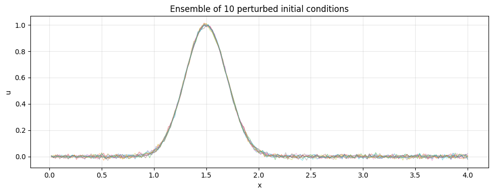

Summary¶

Concept	somax API
Create model	`LinearConvection1D.create(nx=200, Lx=4.0, c=1.0)`
Initial state	`LinearConvection1DState(u=...)`
Forward sim	`model.integrate(state0, t0, t1, dt, saveat=...)`
Diagnostics	`model.diagnose(state)`
Grad w.r.t. params	`eqx.filter_grad(loss)(model)`

Key takeaway: Linear convection translates a signal without distortion. The CFL condition $c \Delta t / \Delta x \le 1$ governs stability.

Next: Step 2 — Nonlinear Convection introduces amplitude-dependent wave speed and shock formation.

Step 1 — 1D Linear Convection