The three extreme-value families

Abstract¶

The single GEV family hides three classical tail types, selected by the sign of the shape parameter ξ: Gumbel (ξ=0, light tail), Fréchet (ξ>0, heavy unbounded tail) and Weibull (ξ<0, bounded tail). This notebook makes the three concrete, then confronts the central difficulty of extreme-value analysis: ξ is weakly identified. We show that all three families fit a real station’s annual maxima almost equally well in-sample, yet imply very different extrapolations; that the Bayesian posterior for ξ straddles zero; and that on short records the estimate ξ̂ swings wildly across the three regimes. The tail type you cannot see is exactly the thing that controls your rarest predictions.

Keywords:GumbelFréchetWeibullshape parameteridentifiability¶

The three faces of the GEV¶

In The GEV distribution the posterior for the shape ξ came out wide and centred near zero. That was not a nuisance — it is the crux of extreme-value analysis. The sign of ξ decides which of three classical distributions the maxima follow, and that decision is precisely the hardest thing to make from data.

Background: one family, three tails¶

Writing the GEV with shape ξ, the limiting form as ξ→0 and the two signed cases are the three types:

\begin{aligned} \textbf{Gumbel } (\xi=0):\quad & G(z)=\exp\!\bigl\{-e^{-(z-\mu)/\sigma}\bigr\}, && z\in\mathbb{R},\\[2pt] \textbf{Fréchet } (\xi>0):\quad & G(z)=\exp\!\bigl\{-[1+\xi\tfrac{z-\mu}{\sigma}]^{-1/\xi}\bigr\}, && z>\mu-\sigma/\xi,\\[2pt] \textbf{Weibull } (\xi<0):\quad & G(z)=\exp\!\bigl\{-[1+\xi\tfrac{z-\mu}{\sigma}]^{-1/\xi}\bigr\}, && z<\mu-\sigma/\xi. \end{aligned}

(1)

The qualitative difference is all in the tail and the support:

Gumbel — light, exponentially decaying upper tail, unbounded.
Fréchet — heavy, polynomial upper tail, unbounded above (a finite lower bound). Extremes can be arbitrarily large.
Weibull — short tail with a finite upper bound $z_{\max}=\mu-\sigma/\xi$ : there is a hard ceiling on the maximum.

For a physical quantity like daily-maximum temperature the question “Gumbel, Fréchet or Weibull?” is the question “is there an effective ceiling, and if not, how heavy is the tail?” — which dominates any long-range prediction.

xtremax provides each type as its own distribution (GumbelType1GEVD, FrechetType2GEVD, WeibullType3GEVD) alongside the unified GeneralizedExtremeValueDistribution.

Setup¶

import sys
import pathlib

try:
    import spatial_extremes  # noqa: F401  already importable (e.g. on PYTHONPATH)
except ModuleNotFoundError:
    _here = pathlib.Path.cwd().resolve()
    _roots = (_here, *_here.parents)
    _cands = [r / "_helpers" for r in _roots]
    _cands += [r / "docs" / "tutorials" / "spatial_extremes" / "_helpers" for r in _roots]
    _src = next((c for c in _cands if (c / "spatial_extremes").exists()), None)
    if _src is None:
        raise RuntimeError("cannot locate docs/tutorials/spatial_extremes/_helpers") from None
    sys.path.insert(0, str(_src))

from __future__ import annotations

import warnings
warnings.filterwarnings("ignore", message=r".*IProgress.*")

import jax
jax.config.update("jax_enable_x64", True)

import numpy as np
import pandas as pd
import jax.numpy as jnp
import jax.random as jr
import matplotlib.pyplot as plt
import seaborn as sns

import numpyro
import numpyro.distributions as ndist
from numpyro.infer import MCMC, NUTS
from numpyro.infer.initialization import init_to_median
import optax

from xtremax import GeneralizedExtremeValueDistribution as GEV
from xtremax import GumbelType1GEVD as Gumbel
from xtremax import FrechetType2GEVD as Frechet
from xtremax import WeibullType3GEVD as Weibull
from xtremax import gev_log_prob

from spatial_extremes import data
from spatial_extremes.places import nearest_city

sns.set_theme(style="whitegrid", context="notebook", palette="deep")

ξ shapes the tail¶

With the same location and scale, the three types diverge only in the tail. Below: their densities, and — more tellingly — their return-level curves (5). The Weibull curve flattens toward its ceiling, Gumbel grows linearly in $\log T$ , and Fréchet accelerates away.

loc0, scale0 = 40.0, 2.5
families = {
    "Gumbel (ξ=0)":    Gumbel(loc=loc0, scale=scale0),
    "Fréchet (ξ=+0.25)": Frechet(loc=loc0, scale=scale0, concentration=0.25),
    "Weibull (ξ=−0.25)": Weibull(loc=loc0, scale=scale0, concentration=-0.25),
}
colors = dict(zip(families, sns.color_palette("deep", 3)))

grid = jnp.linspace(30, 56, 400)
periods = jnp.logspace(np.log10(2), 4, 80)     # up to 10 000 years

fig, (axd, axr) = plt.subplots(1, 2, figsize=(13, 4.8))
for name, dist in families.items():
    axd.plot(grid, jnp.exp(dist.log_prob(grid)), color=colors[name], lw=2, label=name)
    axr.plot(np.asarray(periods), np.asarray(dist.return_level(periods)),
             color=colors[name], lw=2, label=name)
axd.axvline(loc0 + scale0 / 0.25, color=colors["Weibull (ξ=−0.25)"], ls=":", lw=1)
axd.set(xlabel="z (°C)", ylabel="density", title="Densities (same μ, σ)")
axd.legend()
axr.axhline(loc0 + scale0 / 0.25, color=colors["Weibull (ξ=−0.25)"], ls=":", lw=1,
            label="Weibull ceiling")
axr.set_xscale("log")
axr.set(xlabel="return period T (years)", ylabel="return level (°C)",
        title="Return levels fan out with the tail type")
axr.legend()
fig.tight_layout()
plt.show()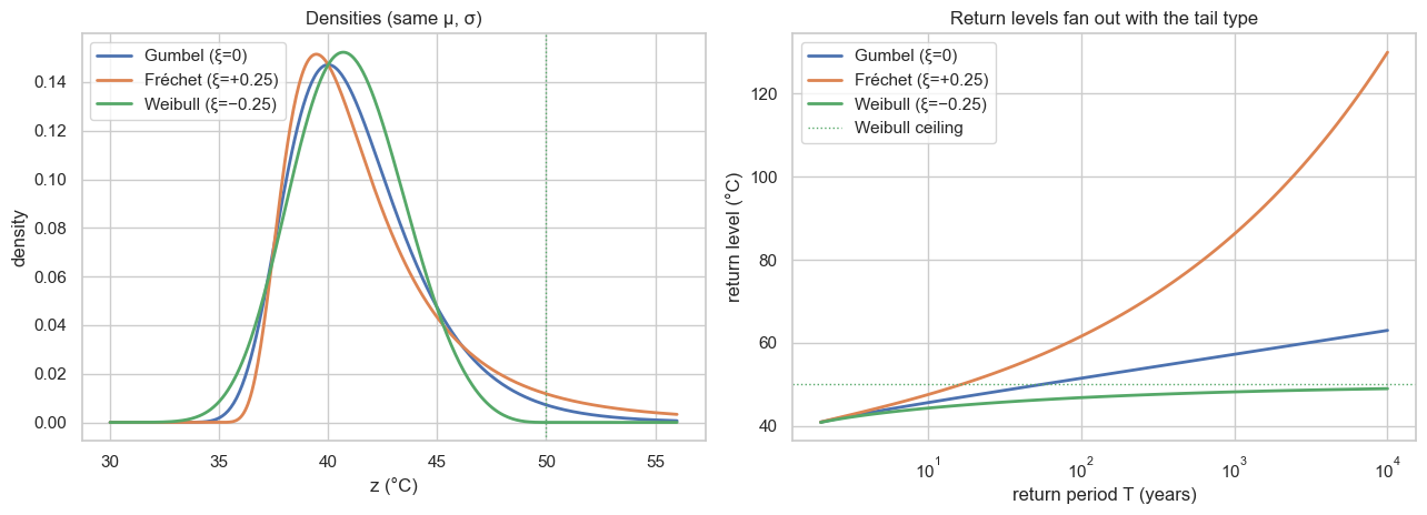

Three families, one dataset¶

Now the empirical puzzle. We take a real station’s annual maxima and fit each type by maximum likelihood, then compare the in-sample fits.

maxima, stations, years, is_real = data.load_annual_maxima(min_periods=300, min_years=20)
order = np.isfinite(maxima).sum(1) + np.nan_to_num(np.nanmean(maxima, axis=1)) / 1e3
sidx = int(np.argmax(order))
lon, lat = float(stations[sidx, 0]), float(stations[sidx, 1])
city, dist0 = nearest_city(lon, lat)
place = city if dist0 < 12 else f"near {city}"
m_ = np.isfinite(maxima[sidx])
y = jnp.asarray(maxima[sidx][m_]); y_np = np.asarray(y); m = y_np.size
print("source:", "REAL CDS" if is_real else "synthetic", "| station:", place,
      f"({m} annual maxima)")


def mle(neg_log_lik, init, steps=800):
    opt = optax.adam(0.05); state = opt.init(init)
    def step(carry, _):
        p, state = carry
        g = jax.grad(neg_log_lik)(p)
        upd, state = opt.update(g, state, p)
        return (optax.apply_updates(p, upd), state), None
    (p, _), _ = jax.lax.scan(step, (init, state), None, length=steps)
    return p

ymean, ystd, lystd = float(y.mean()), float(y.std()), float(jnp.log(y.std()))

def nll_gum(p):
    mu, ls = p
    return -Gumbel(loc=mu, scale=jnp.exp(ls)).log_prob(y).sum()
def nll_fre(p):
    mu, ls, lx = p
    return -Frechet(loc=mu, scale=jnp.exp(ls), concentration=jnp.exp(lx)).log_prob(y).sum()
def nll_wei(p):
    mu, ls, lx = p
    return -Weibull(loc=mu, scale=jnp.exp(ls), concentration=-jnp.exp(lx)).log_prob(y).sum()

pg = mle(nll_gum, (jnp.array(ymean), jnp.array(lystd)))
pf = mle(nll_fre, (jnp.array(ymean), jnp.array(lystd), jnp.array(np.log(0.1))))
pw = mle(nll_wei, (jnp.array(ymean), jnp.array(lystd), jnp.array(np.log(0.1))))

fits = {
    "Gumbel":  (Gumbel(loc=pg[0], scale=jnp.exp(pg[1])), 2, -float(nll_gum(pg)), 0.0),
    "Fréchet": (Frechet(loc=pf[0], scale=jnp.exp(pf[1]), concentration=jnp.exp(pf[2])),
                3, -float(nll_fre(pf)), float(jnp.exp(pf[2]))),
    "Weibull": (Weibull(loc=pw[0], scale=jnp.exp(pw[1]), concentration=-jnp.exp(pw[2])),
                3, -float(nll_wei(pw)), -float(jnp.exp(pw[2]))),
}
fam_colors = dict(zip(fits, sns.color_palette("deep", 3)))

source: REAL CDS | station: near Zaragoza (120 annual maxima)

In-sample, they are nearly indistinguishable — the fitted densities lie almost on top of one another, and the goodness-of-fit scores barely differ:

zs = np.sort(y_np)
p_emp = (np.arange(1, m + 1) - 0.5) / m
gx = jnp.linspace(zs.min() - 2, zs.max() + 4, 300)

fig, ax = plt.subplots(figsize=(7, 4.4))
ax.hist(y_np, bins=12, density=True, color="0.8", label="annual maxima")
rows = []
for name, (dist, k, logL, xi) in fits.items():
    ax.plot(gx, jnp.exp(dist.log_prob(gx)), color=fam_colors[name], lw=2, label=name)
    ks = float(np.max(np.abs(np.asarray(dist.cdf(jnp.asarray(zs))) - p_emp)))
    rows.append((name, xi, logL, 2 * k - 2 * logL, ks))
ax.set(xlabel="°C", ylabel="density", title=f"{place}: three families, one dataset")
ax.legend()
plt.show()

gof = pd.DataFrame(rows, columns=["family", "ξ̂", "log-lik", "AIC", "KS"]).set_index("family")
print(gof.round(3).to_string())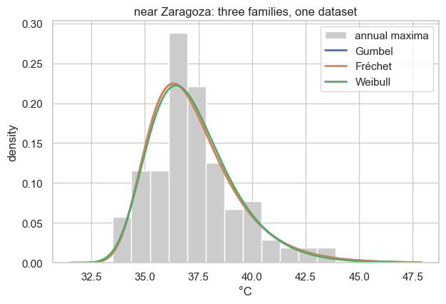

            ξ̂  log-lik      AIC     KS
family                                 
Gumbel   0.000 -246.942  497.883  0.068
Fréchet  0.001 -246.953  499.905  0.068
Weibull -0.047 -246.662  499.324  0.075

...but they predict different extremes¶

The catch appears only when we extrapolate. The same three fitted models — indistinguishable on the data — diverge at long return periods: Weibull bends to its finite ceiling while Fréchet/Gumbel keep climbing. The choice of tail type we could not make from the data is the choice that sets the rarest design values.

periods = jnp.logspace(np.log10(2), 4, 80)
emp_T = 1.0 / (1.0 - (np.arange(1, m + 1) - 0.44) / (m + 0.12))

fig, ax = plt.subplots(figsize=(8, 5))
for name, (dist, *_) in fits.items():
    ax.plot(np.asarray(periods), np.asarray(dist.return_level(periods)),
            color=fam_colors[name], lw=2, label=name)
ax.scatter(emp_T, zs, color="k", s=24, zorder=5, label="observed maxima")
ax.set_xscale("log")
ax.set(xlabel="return period T (years)", ylabel="return level (°C)",
       title=f"{place}: identical fits, divergent extrapolations")
ax.legend()
plt.show()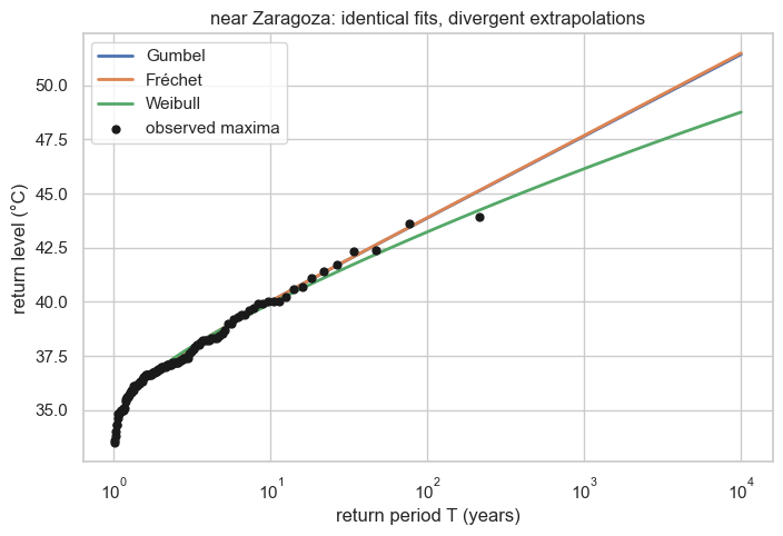

The shape parameter is weakly identified¶

Why can’t the data choose? Because $\xi$ is weakly identified from a few dozen maxima. Two views make this concrete.

Bayesian. The full-GEV posterior for $\xi$ straddles zero, putting real mass in all three regimes — so the data are genuinely consistent with Gumbel, Fréchet and Weibull.

def gev_model(obs):
    mu = numpyro.sample("mu", ndist.Normal(ymean, 5.0))
    sigma = numpyro.sample("sigma", ndist.HalfNormal(ystd))
    xi = numpyro.sample("xi", ndist.Normal(0.0, 0.25))
    numpyro.sample("obs", GEV(loc=mu, scale=sigma, concentration=xi), obs=obs)

mcmc = MCMC(NUTS(gev_model, target_accept_prob=0.95, init_strategy=init_to_median),
            num_warmup=1500, num_samples=2000, num_chains=2,
            chain_method="vectorized", progress_bar=False)
mcmc.run(jr.PRNGKey(0), y)
xi_post = np.asarray(mcmc.get_samples()["xi"])
p_neg, p_zero, p_pos = (np.mean(xi_post < -0.05),
                        np.mean(np.abs(xi_post) <= 0.05),
                        np.mean(xi_post > 0.05))

fig, ax = plt.subplots(figsize=(7.5, 4))
sns.histplot(xi_post, bins=50, stat="density", color="0.6", ax=ax)
for lo, hi, c, lab in [(-1, -0.05, fam_colors["Weibull"], f"Weibull  {p_neg:.0%}"),
                       (-0.05, 0.05, fam_colors["Gumbel"], f"~Gumbel  {p_zero:.0%}"),
                       (0.05, 1, fam_colors["Fréchet"], f"Fréchet  {p_pos:.0%}")]:
    ax.axvspan(lo, hi, color=c, alpha=0.12)
    ax.plot([], [], color=c, lw=8, alpha=0.4, label=lab)
ax.axvline(0, color="k", lw=1)
ax.set(xlim=(xi_post.min() - 0.05, xi_post.max() + 0.05), xlabel="shape ξ",
       ylabel="posterior density", title=f"{place}: posterior of ξ spans all three types")
ax.legend(title="posterior mass")
plt.show()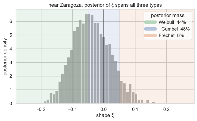

Frequentist / small-sample. Even when the truth is a definite type, a short record cannot recover it. We simulate many records of the same length from a known mildly-Fréchet GEV ( $\xi=0.15$ ) and re-estimate $\xi$ each time: the sampling distribution of $\hat\xi$ is broad and routinely crosses into the wrong regime.

xi_true, n_rep = 0.15, 400
truth = GEV(loc=40.0, scale=2.5, concentration=xi_true)
sims = truth.sample(jr.PRNGKey(1), (n_rep, m))      # (n_rep, m) synthetic records

def fit_xi(sample):
    s_mean, s_lstd = jnp.mean(sample), jnp.log(jnp.std(sample))
    def nll(p):
        mu, ls, xi = p
        return -gev_log_prob(sample, mu, jnp.exp(ls), xi).sum()
    p = mle(nll, (s_mean, s_lstd, jnp.array(0.0)))
    return p[2]

xi_hat = np.asarray(jax.vmap(fit_xi)(sims))
frac_wrong_sign = float(np.mean(xi_hat < 0))

fig, ax = plt.subplots(figsize=(7.5, 4))
sns.histplot(xi_hat, bins=40, stat="density", color="0.6", ax=ax)
ax.axvline(xi_true, color="#C44E52", lw=2, label=f"true ξ = {xi_true}")
ax.axvline(0, color="k", lw=1, ls="--", label="Gumbel boundary")
ax.set(xlabel="estimated ξ̂", ylabel="density",
       title=f"ξ̂ from {m}-year records (truth ξ={xi_true}): "
             f"{frac_wrong_sign:.0%} land below 0")
ax.legend()
plt.show()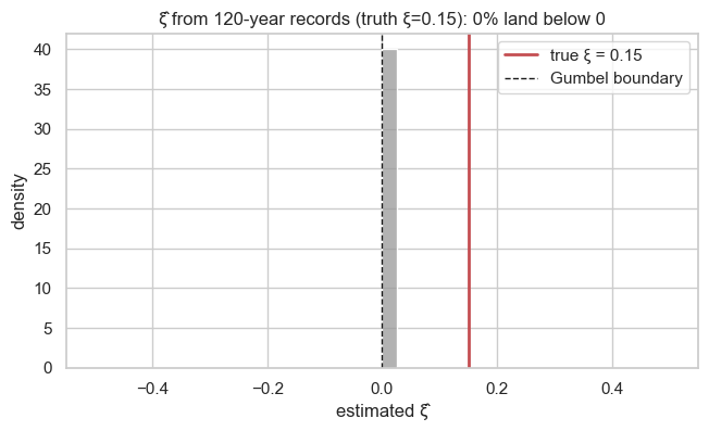

Recap & where next¶

The GEV’s three faces — Gumbel, Fréchet, Weibull — are selected by the sign of $\xi$ , and that sign governs whether extremes are bounded and how heavy the tail is. Yet $\xi$ is weakly identified: families that are indistinguishable on a station’s record imply sharply different rare-event predictions, the posterior for $\xi$ spans all three types, and short-record estimates $\hat\xi$ scatter across the boundary.

This is the core motivation for the rest of the curriculum. A single station simply does not contain enough extremes to fix its tail. The fix is to borrow strength across space: neighbouring stations share a climate, so pooling their maxima through a spatial Gaussian process sharpens $\xi$ (and every return level that depends on it). We build toward that next, starting by fitting every station independently in Every station on its own to see the noise we need to tame.