Inhomogeneous Spatial Poisson Process — From Scratch and With NumPyro

An inhomogeneous spatial Poisson process (IPP) on a domain $D \subset \mathbb{R}^d$ has a non-constant intensity $\lambda(s) \geq 0$ . The total expected count is the integrated intensity

\Lambda(D) = \int_D \lambda(s)\, ds,

(1)

the count is $N \sim \mathrm{Poisson}(\Lambda)$ , and the joint log-likelihood factorises as

\log L = \sum_{i=1}^n \log \lambda(s_i) - \Lambda(D).

(2)

Inhomogeneity is the bread and butter of applied spatial statistics: disease incidence around risk factors, earthquake epicentres along fault lines, methane plumes near industrial facilities, galaxies in the cosmic web. This notebook walks through the same two faces of xtremax as the homogeneous case.

From scratch — primitives for sampling (Lewis–Shedler thinning), evaluating the joint log-likelihood, and integrating the intensity over the box (trapezoid grid + Halton QMC).
With NumPyro — wrap the IPP as a Distribution and run NUTS to recover hyperparameters of a Gaussian-bump intensity field.

Setup¶

%pip install -q xtremax matplotlib  # uncomment on Colab
import jax.numpy as jnp
import matplotlib.pyplot as plt
import numpyro
import numpyro.distributions as dist
from jax import random
from jax.scipy.stats import norm
from numpyro.infer import MCMC, NUTS

from xtremax.point_processes import (
    RectangularDomain,
    integrate_log_intensity_spatial,
)
from xtremax.point_processes.distributions import (
    InhomogeneousSpatialPP as IppSpatialDist,
)
from xtremax.point_processes.primitives import (
    ipp_spatial_log_prob,
    ipp_spatial_sample_thinning,
)


plt.rcParams["figure.figsize"] = (8.0, 4.0)

/home/azureuser/localfiles/xtremax/.venv/bin/python: No module named pip

Note: you may need to restart the kernel to use updated packages.

/home/azureuser/localfiles/xtremax/.venv/lib/python3.13/site-packages/tqdm/auto.py:21: TqdmWarning: IProgress not found. Please update jupyter and ipywidgets. See https://ipywidgets.readthedocs.io/en/stable/user_install.html
  from .autonotebook import tqdm as notebook_tqdm

1. From scratch — the primitives layer¶

Start with a single Gaussian bump centred at the middle of a $[0, 10]^2$ domain. The log-intensity is a quadratic in space, so it has a tidy closed form for the integrated intensity (which we’ll use to sanity-check the quadrature primitive).

domain = RectangularDomain.from_size(jnp.array([10.0, 10.0]))


def log_intensity(s):
    # Smooth bump: λ(s) = 5 · exp(-0.5 ||s - 5||²). Peak intensity is 5.
    return jnp.log(5.0) - 0.5 * jnp.sum((s - 5.0) ** 2, axis=-1)


# Visualise the field on a grid.
xy = jnp.linspace(0, 10, 80)
X, Y = jnp.meshgrid(xy, xy)
grid = jnp.stack([X.ravel(), Y.ravel()], axis=-1)
intensity = jnp.exp(log_intensity(grid)).reshape(X.shape)

fig, ax = plt.subplots(figsize=(5, 4.5))
im = ax.imshow(intensity, extent=[0, 10, 0, 10], origin="lower", cmap="viridis")
plt.colorbar(im, label="λ(s)")
ax.set_xlabel("x")
ax.set_ylabel("y")
ax.set_title("Intensity field λ(s)")
plt.tight_layout()
plt.show()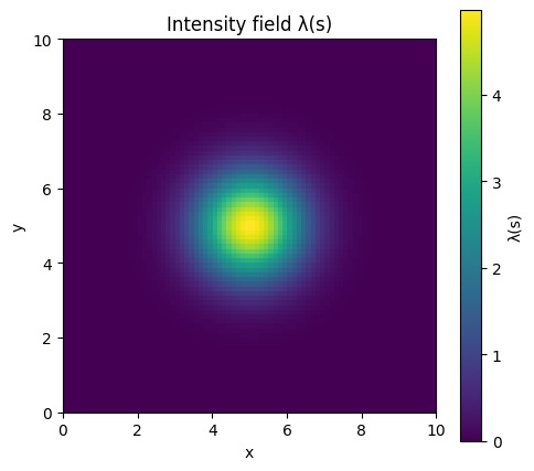

Integrated intensity¶

integrate_log_intensity_spatial computes $\Lambda(D)$ on the rectangular domain. Two methods: tensor-product trapezoid (best for $d \leq 2$ and smooth integrands) and Halton QMC (better for $d \geq 3$ , robust to peaks). We compare against the analytical answer.

# Closed form: ∫∫ 5 · exp(-½ ((x-5)² + (y-5)²)) dx dy
#            = 5 · (∫_0^{10} exp(-½ (x-5)²) dx)²
#            = 5 · (√(2π) · (Φ(5) - Φ(-5)))²,  where Φ = standard normal CDF.
per_axis = jnp.sqrt(2.0 * jnp.pi) * (norm.cdf(5.0) - norm.cdf(-5.0))
exact = 5.0 * per_axis**2
trap = integrate_log_intensity_spatial(
    log_intensity, domain, n_points=4096, method="trapezoid"
)
qmc = integrate_log_intensity_spatial(
    log_intensity, domain, n_points=4096, method="qmc"
)
print(f"Analytical Λ(D)  = {float(exact):.4f}")
print(f"Trapezoid (4096) = {float(trap):.4f}")
print(f"QMC       (4096) = {float(qmc):.4f}")

Analytical Λ(D)  = 31.4159
Trapezoid (4096) = 31.4159
QMC       (4096) = 31.4339

Sampling — Lewis–Shedler thinning¶

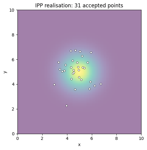
Sampling an IPP requires a thinning bound $\lambda_{\max} \geq \max_s \lambda(s)$ over the box. Procedure: draw an HPP at rate $\lambda_{\max}$ over $D$ , then accept each candidate with probability $\lambda(s)/\lambda_{\max}$ . Tighter bounds give higher acceptance.

lambda_max = 5.0  # tight: peak intensity exactly 5.
locs, accepted, n_uncapped = ipp_spatial_sample_thinning(
    random.PRNGKey(0),
    log_intensity,
    domain,
    lambda_max=lambda_max,
    max_candidates=1024,
)
print(
    f"Drew {int(n_uncapped)} candidates, {int(accepted.sum())} accepted "
    f"(acceptance ≈ {float(accepted.sum() / n_uncapped):.2%})"
)

fig, ax = plt.subplots(figsize=(5, 5))
ax.imshow(intensity, extent=[0, 10, 0, 10], origin="lower", cmap="viridis", alpha=0.5)
real_locs = locs[accepted]
ax.scatter(
    real_locs[:, 0],
    real_locs[:, 1],
    s=18,
    color="white",
    edgecolors="black",
    linewidth=0.5,
)
ax.set_xlim(0, 10)
ax.set_ylim(0, 10)
ax.set_aspect("equal")
ax.set_title(f"IPP realisation: {int(accepted.sum())} accepted points")
ax.set_xlabel("x")
ax.set_ylabel("y")
plt.tight_layout()
plt.show()

Drew 467 candidates, 31 accepted (acceptance ≈ 6.64%)

Joint log-likelihood¶

The decomposition $\log L = \sum \log \lambda(s_i) - \Lambda(D)$ is implemented directly. A useful diagnostic: drag the candidate parameters away from the truth and watch the log-likelihood drop.

log_p_truth = ipp_spatial_log_prob(locs, accepted, log_intensity, exact)
print(f"log L at truth = {float(log_p_truth):.2f}")


# A misspecified intensity (peak shifted to (8, 8)) should score lower.
def shifted_log_intensity(s):
    return jnp.log(5.0) - 0.5 * jnp.sum((s - 8.0) ** 2, axis=-1)


lambda_shifted = integrate_log_intensity_spatial(
    shifted_log_intensity, domain, n_points=4096, method="qmc"
)
log_p_shift = ipp_spatial_log_prob(
    locs, accepted, shifted_log_intensity, lambda_shifted
)
print(f"log L at shifted peak = {float(log_p_shift):.2f}")

log L at truth = -10.37
log L at shifted peak = -303.70

2. With NumPyro — Bayesian inference for the intensity peak¶

Treat the centre and amplitude of the Gaussian bump as latent and recover them from the observed pattern. The wrapper class InhomogeneousSpatialPP integrates Λ(D) on every log_prob call so gradients flow into both the sum-of-log-intensities and the $-\Lambda$ term.

# Synthetic observation with a known peak.
true_centre = jnp.array([4.0, 6.0])
true_log_amp = jnp.log(5.0)


def true_log_intensity(s):
    return true_log_amp - 0.5 * jnp.sum((s - true_centre) ** 2, axis=-1)


obs_locs, obs_mask, _ = ipp_spatial_sample_thinning(
    random.PRNGKey(7),
    true_log_intensity,
    domain,
    lambda_max=5.0,
    max_candidates=1024,
)
print(f"Observed {int(obs_mask.sum())} points")

Observed 38 points

# Score the heterogeneous ``(locations, mask)`` PyTree via ``numpyro.factor``
# rather than ``numpyro.sample(..., obs=...)`` — see the HPP spatial
# notebook for the full rationale.
def model():
    centre = numpyro.sample("centre", dist.Normal(jnp.full(2, 5.0), 2.0))
    log_amp = numpyro.sample("log_amp", dist.Normal(0.0, 1.5))

    def log_lam(s):
        return log_amp - 0.5 * jnp.sum((s - centre) ** 2, axis=-1)

    spp = IppSpatialDist(
        log_lam,
        domain=domain,
        lambda_max=10.0,
        max_candidates=1024,
        n_integration_points=2048,
    )
    numpyro.factor("lik", spp.log_prob((obs_locs, obs_mask)))


mcmc = MCMC(
    NUTS(model),
    num_warmup=500,
    num_samples=1000,
    progress_bar=False,
)
mcmc.run(random.PRNGKey(0))
mcmc.print_summary()


                mean       std    median      5.0%     95.0%     n_eff     r_hat
 centre[0]      3.82      0.16      3.81      3.59      4.10   1157.76      1.00
 centre[1]      5.80      0.17      5.80      5.55      6.08    899.85      1.00
   log_amp      1.78      0.17      1.78      1.51      2.05    748.53      1.00

Number of divergences: 0

Posterior should concentrate around the true peak location $(4, 6)$ and amplitude $\log 5 \approx 1.61$ .

samples = mcmc.get_samples()
fig, axes = plt.subplots(1, 3, figsize=(12, 3.5))

for ax, key, truth in zip(
    axes[:2],
    ("centre x", "centre y"),
    (float(true_centre[0]), float(true_centre[1])),
    strict=False,
):
    coord = 0 if "x" in key else 1
    ax.hist(samples["centre"][:, coord], bins=40, alpha=0.75, density=True)
    ax.axvline(truth, color="k", linestyle="--", label=f"truth = {truth}")
    ax.set_title(f"posterior over {key}")
    ax.legend()

axes[2].hist(samples["log_amp"], bins=40, alpha=0.75, density=True)
axes[2].axvline(
    float(true_log_amp),
    color="k",
    linestyle="--",
    label=f"truth = {float(true_log_amp):.2f}",
)
axes[2].set_title("posterior over log amplitude")
axes[2].legend()
plt.tight_layout()
plt.show()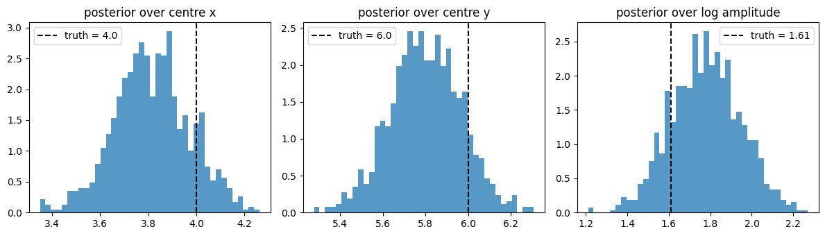

3. Higher dimensions — same API¶

The whole pipeline scales to 3-D without code changes — only domain_size grows by one entry.

domain_3d = RectangularDomain.from_size(jnp.array([4.0, 4.0, 4.0]))


def log_intensity_3d(s):
    return jnp.log(2.0) - 0.5 * jnp.sum((s - 2.0) ** 2, axis=-1)


lam_d3 = integrate_log_intensity_spatial(
    log_intensity_3d, domain_3d, n_points=8192, method="qmc"
)
print(f"3-D Λ(D) ≈ {float(lam_d3):.3f}")

locs_3d, mask_3d, _ = ipp_spatial_sample_thinning(
    random.PRNGKey(0), log_intensity_3d, domain_3d, lambda_max=2.0, max_candidates=512
)
print(f"3-D realisation: {int(mask_3d.sum())} points in 4³ box")

3-D Λ(D) ≈ 27.393

3-D realisation: 23 points in 4³ box

Where to go from here¶

Marked spatial patterns. Pair each event with a magnitude — see the Marked Spatial PP notebook.
Tighter quadrature. For sharply peaked intensities, increase n_integration_points or pass an analytical $\Lambda$ via the operator’s integrated_intensity= argument.
Neural intensities. Replace the analytical bump with an eqx.Module (e.g. a small MLP). Its parameters become PyTree leaves and gradients flow through log_prob.