Marked Spatial Point Process — From Scratch and With NumPyro

A marked spatial point process pairs each event location with a mark — a magnitude, type, size, or any other random attribute attached to the point. Common examples:

tree locations + diameters,
earthquake epicentres + magnitudes (Gutenberg–Richter),
crime events + severity codes,
methane plumes + emission rates.

Under the separable factorisation $\lambda(s, m) = \lambda(s)\, f(m \mid s)$ , the joint log-likelihood splits into a ground-process term and a mark term:

\log L = \sum_{i=1}^n \log \lambda(s_i) + \sum_{i=1}^n \log f(m_i \mid s_i) - \Lambda(D).

(1)

xtremax’s MarkedSpatialPP is exactly this: a ground operator (homogeneous or inhomogeneous spatial PP) plus a user-supplied mark distribution callable. Marks can be scalar, vector, discrete, or location-dependent — anything a numpyro.distributions.Distribution can express.

Setup¶

%pip install -q xtremax matplotlib  # uncomment on Colab
import jax.numpy as jnp
import matplotlib.pyplot as plt
import numpyro
import numpyro.distributions as dist
from jax import random
from numpyro.infer import MCMC, NUTS

from xtremax.point_processes import RectangularDomain
from xtremax.point_processes.distributions import (
    MarkedSpatialPP as MarkedSpatialDist,
)
from xtremax.point_processes.operators import (
    HomogeneousSpatialPP,
    InhomogeneousSpatialPP,
    MarkedSpatialPP,
)


plt.rcParams["figure.figsize"] = (8.0, 4.0)

/home/azureuser/localfiles/xtremax/.venv/bin/python: No module named pip

Note: you may need to restart the kernel to use updated packages.

/home/azureuser/localfiles/xtremax/.venv/lib/python3.13/site-packages/tqdm/auto.py:21: TqdmWarning: IProgress not found. Please update jupyter and ipywidgets. See https://ipywidgets.readthedocs.io/en/stable/user_install.html
  from .autonotebook import tqdm as notebook_tqdm

1. Independent marks: trees with random diameters¶

The simplest marked process: locations from a homogeneous spatial PP, marks i.i.d. Gamma. The mark distribution callable ignores its input and just returns the same Gamma for every event.

domain = RectangularDomain.from_size(jnp.array([10.0, 10.0]))  # 10m × 10m plot
ground = HomogeneousSpatialPP(rate=0.5, domain=domain)
diameter_dist = dist.Gamma(concentration=5.0, rate=2.0)  # mean = 2.5, variance = 1.25

trees = MarkedSpatialPP(
    ground=ground,
    mark_distribution_fn=lambda s: diameter_dist,  # location-independent
)

locs, mask, diameters = trees.sample(random.PRNGKey(0), max_events=128)
print(
    f"Sampled {int(mask.sum())} trees, mean diameter = {float(jnp.mean(diameters[mask])):.2f} m"
)

Sampled 38 trees, mean diameter = 2.59 m

fig, ax = plt.subplots(figsize=(5, 5))
real_locs = locs[mask]
real_diameters = diameters[mask]
sc = ax.scatter(
    real_locs[:, 0],
    real_locs[:, 1],
    s=20 * real_diameters**2,
    c=real_diameters,
    cmap="viridis",
    alpha=0.8,
    edgecolors="black",
    linewidth=0.4,
)
plt.colorbar(sc, label="diameter (m)")
ax.set_xlim(0, 10)
ax.set_ylim(0, 10)
ax.set_aspect("equal")
ax.set_xlabel("x (m)")
ax.set_ylabel("y (m)")
ax.set_title("Trees: locations + diameters")
plt.tight_layout()
plt.show()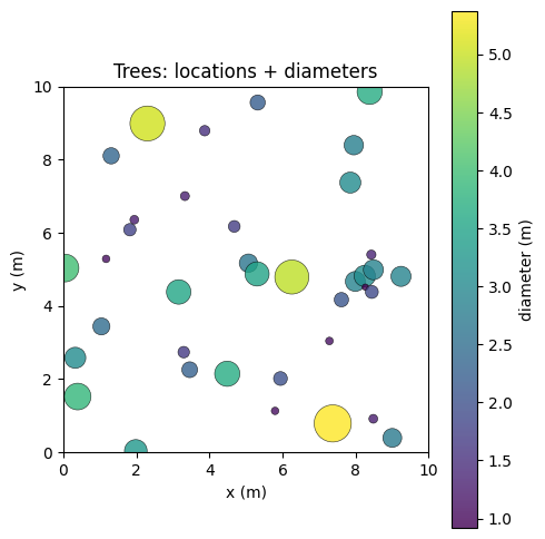

The joint log-likelihood decomposes — and we can score the ground and mark terms separately.

joint_lp = trees.log_prob(locs, mask, diameters)
ground_lp = trees.ground_log_prob(locs, mask)
marks_lp = trees.marks_log_prob(locs, diameters, mask)
print(
    f"joint log L = {float(joint_lp):.2f}  =  ground {float(ground_lp):.2f} + marks {float(marks_lp):.2f}"
)
assert jnp.allclose(joint_lp, ground_lp + marks_lp)

joint log L = -308.11  =  ground -251.34 + marks -56.77

2. Location-dependent marks: earthquakes along a fault line¶

Now make the mark law depend on space. Earthquake magnitudes follow Gutenberg–Richter — Exponential with a $b$ -value parameter — but suppose the $b$ -value is smaller (heavier-tailed magnitudes) closer to the fault. We’ll use an inhomogeneous spatial PP whose intensity is concentrated along a diagonal fault, and an Exponential mark with rate inversely proportional to distance from that fault.

fault_domain = RectangularDomain.from_size(jnp.array([100.0, 100.0]))  # 100km × 100km


def fault_log_intensity(s):
    # Fault line: y = x. Distance from the line: |x - y| / √2.
    dist_to_fault = jnp.abs(s[..., 0] - s[..., 1]) / jnp.sqrt(2.0)
    # Higher rate near the fault.
    return jnp.log(0.05 + 0.5 * jnp.exp(-0.05 * dist_to_fault))


fault_pp = InhomogeneousSpatialPP(
    fault_log_intensity, fault_domain, lambda_max=0.55, n_integration_points=4096
)


def magnitude_dist(s):
    # b-value smaller (higher-magnitude events more likely) near the fault.
    dist_to_fault = jnp.abs(s[0] - s[1]) / jnp.sqrt(2.0)
    b_value = (
        1.0 + 0.5 * dist_to_fault / 50.0
    )  # b ranges from 1 (on fault) to ~1.7 (far)
    return dist.Exponential(rate=b_value)


earthquakes = MarkedSpatialPP(
    ground=fault_pp,
    mark_distribution_fn=magnitude_dist,
)

eq_locs, eq_mask, eq_mags = earthquakes.sample(random.PRNGKey(2), max_events=2048)
print(
    f"Sampled {int(eq_mask.sum())} earthquakes, max magnitude = {float(jnp.max(eq_mags)):.2f}"
)

Sampled 932 earthquakes, max magnitude = 7.03

fig, ax = plt.subplots(figsize=(6, 5.5))
real_eq_locs = eq_locs[eq_mask]
real_mags = eq_mags[eq_mask]
sc = ax.scatter(
    real_eq_locs[:, 0],
    real_eq_locs[:, 1],
    s=10 + 50 * real_mags,
    c=real_mags,
    cmap="hot",
    alpha=0.7,
    edgecolors="black",
    linewidth=0.2,
)
plt.colorbar(sc, label="magnitude")
# Overlay the fault line.
ax.plot([0, 100], [0, 100], "k--", alpha=0.4, label="fault line")
ax.set_xlim(0, 100)
ax.set_ylim(0, 100)
ax.set_aspect("equal")
ax.set_xlabel("x (km)")
ax.set_ylabel("y (km)")
ax.set_title("Earthquake epicentres + magnitudes (location-dependent b-value)")
ax.legend(loc="upper left")
plt.tight_layout()
plt.show()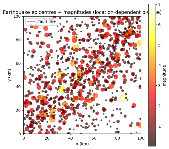

Sanity check: events near the fault should have higher mean magnitude than events far from it (lower b-value → heavier tail).

real_dists = jnp.abs(real_eq_locs[:, 0] - real_eq_locs[:, 1]) / jnp.sqrt(2.0)
near_fault = real_mags[real_dists < 10.0]
far_fault = real_mags[real_dists > 30.0]
print(f"Mean magnitude within 10 km of fault: {float(jnp.mean(near_fault)):.3f}")
print(f"Mean magnitude beyond 30 km of fault: {float(jnp.mean(far_fault)):.3f}")

Mean magnitude within 10 km of fault: 0.851
Mean magnitude beyond 30 km of fault: 0.695

3. With NumPyro — joint inference over ground rate and mark scale¶

Treat both the ground rate $\lambda$ and the mark scale parameter as latent. The joint log-likelihood means a single NUTS run gives us a coherent posterior over both.

true_rate = 0.4
true_concentration = 4.0
true_mark_rate = 1.5
ground_synth = HomogeneousSpatialPP(rate=true_rate, domain=domain)
mark_synth = dist.Gamma(concentration=true_concentration, rate=true_mark_rate)
synth_pp = MarkedSpatialPP(
    ground=ground_synth, mark_distribution_fn=lambda s: mark_synth
)
obs_locs, obs_mask, obs_marks = synth_pp.sample(random.PRNGKey(0), max_events=128)
print(f"Synthetic observation: {int(obs_mask.sum())} events")

Synthetic observation: 29 events

# Score via ``numpyro.factor`` since the observation is a heterogeneous
# PyTree ``(locations, mask, marks)`` rather than a single array.
def model():
    rate = numpyro.sample("rate", dist.LogNormal(0.0, 1.0))
    mark_concentration = numpyro.sample(
        "mark_concentration", dist.LogNormal(jnp.log(4.0), 0.5)
    )
    mark_rate = numpyro.sample("mark_rate", dist.LogNormal(jnp.log(1.5), 0.5))

    ground = HomogeneousSpatialPP(rate=rate, domain=domain)
    mpp = MarkedSpatialDist(
        ground=ground,
        mark_distribution_fn=lambda s: dist.Gamma(
            concentration=mark_concentration, rate=mark_rate
        ),
        max_events=128,
    )
    numpyro.factor("lik", mpp.log_prob((obs_locs, obs_mask, obs_marks)))


mcmc = MCMC(NUTS(model), num_warmup=500, num_samples=1000, progress_bar=False)
mcmc.run(random.PRNGKey(0))
mcmc.print_summary()


                          mean       std    median      5.0%     95.0%     n_eff     r_hat
  mark_concentration      4.06      0.89      3.99      2.78      5.60    291.15      1.00
           mark_rate      1.42      0.33      1.39      0.89      1.91    293.28      1.00
                rate      0.30      0.06      0.30      0.21      0.39    539.76      1.00

Number of divergences: 0

All three posteriors should concentrate near the truth. The ground rate is informed only by the count, the Gamma parameters only by the magnitudes — the separable factorisation makes each subset of parameters an essentially independent posterior block (modulo whatever prior coupling we impose).

samples = mcmc.get_samples()
truths = {
    "rate": true_rate,
    "mark_concentration": true_concentration,
    "mark_rate": true_mark_rate,
}
fig, axes = plt.subplots(1, 3, figsize=(12, 3.5))
for ax, name in zip(axes, ("rate", "mark_concentration", "mark_rate"), strict=False):
    ax.hist(samples[name], bins=40, alpha=0.75, density=True)
    ax.axvline(truths[name], color="k", linestyle="--", label=f"truth = {truths[name]}")
    ax.set_title(f"posterior over {name}")
    ax.legend()
plt.tight_layout()
plt.show()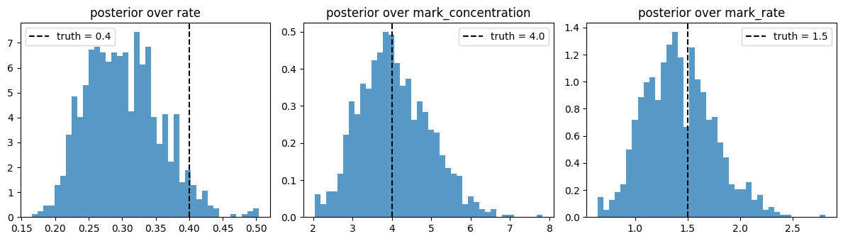

Where to go from here¶

Vector or discrete marks. Swap the mark distribution for MultivariateNormal (vector marks), Categorical (event types), or Pareto (heavy-tailed magnitudes). The factorisation and the API don’t change.
Joint posterior over intensity and mark hyperparameters. Using InhomogeneousSpatialPP as the ground process, you can infer both the spatial peak location and a magnitude-decay rate in a single NUTS run.
Higher dimensions. As with the unmarked spatial PPs, mark inference works for $d \in \{1, 2, 3, \ldots\}$ — the mark distribution callable just consumes the location’s full $d$ -vector.