functax: function approximation for JAX
functax is the stack’s function-approximation library: one representation, f̂(x) = Σⱼ cⱼ φⱼ(x; θ), and five operations on it, namely interpolate, differentiate, integrate, project and transform. It sits at Core tier 0 on JAX, Equinox, lineax and einx alone, takes over geonnax’s bases, and replaces interpax and orthax outright. Status: proposed. Interpolation is designed in depth below; the other modules are in outline.
At a glance
| Layer, tier | Core, tier 0 |
| Imports | NumPy in the base install; JAX, Equinox, lineax and einx in the functax[jax] extra, which every module except the affine kernels needs (decisions 16 and 17) |
| Imported by | every layer above: GeoStack, GeoNumerics, GeoModels, and Core libraries at tier 1 and up |
| Replaces | interpax and orthax, outright; the stack’s hand-rolled bilinear samplers |
| Takes over | geonnax’s bases, sphere grids, transforms and field derivatives |
| Status | proposed; no repository yet |
| Tracked in | the layer map; the role ladder in geostack#122 |
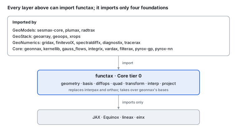
Where functax sits · core tier 0.
functax sits just above the foundations, so every library that needs a basis, a grid sampler or a quadrature rule can import it without breaking the layer rule.
This page is the design: what functax is, how it is used and what is decided. The implementation reference (building blocks, core types, the eleven algorithm patterns, JAX notes and the code survey) is in functax: design details.
The problem and the factorisation
Interpolation takes samples y at sites X, builds a field f̂, and reads it at new sites X*. Every scheme worth supporting fits one four-step pattern.
Geometry. Where the samples and the targets live: a 1-D axis, a regular or rectilinear grid, a curvilinear grid, scattered points, the sphere.
Basis φⱼ. What the field is built from: hat functions, cubic kernels, B-splines, radial kernels, grid cells, a network.
Fit 𝒮. A solver from data to coefficients. Local schemes use the identity, so c = y.
Evaluate H. A matrix from coefficients to target values, sparse for local bases. Its adjoint Hᵀ is a scatter-add back onto the sources.
Read through this pattern, the schemes differ in only two places: the stencil inside H, and the solver 𝒮.
| Scheme | Basis φⱼ | Fit 𝒮 | Read-out H |
|---|---|---|---|
| Nearest | indicator of the cell | identity | 1 tap per row |
| Linear, bilinear, trilinear | hat | identity | 2ᵈ taps per row |
| Cubic convolution (Keys) | piecewise cubic kernel | identity | 4ᵈ taps per row |
| B-spline of order k | B-spline | banded prefilter | (k+1)ᵈ taps per row |
| 1-D cubic spline | piecewise cubic | tridiagonal solve | 4 taps per row |
| PCHIP, Akima, Steffen | Hermite cubic | slopes from y, nonlinear | 4 taps, weights depend on y |
| Inverse distance | none, weights only | identity | k neighbours per row |
| RBF | kernel k(x, xⱼ) | (K + λI) c = y | dense, or sparse with compact kernels |
| Kriging, GP | kernel plus drift | GP solve | dense; adds a variance |
| Smoothing, variational | grid cells | (HᵀR⁻¹H + λLᵀL) x = HᵀR⁻¹y | identity on the grid |
| Neural field | network | gradient descent | nonlinear in c |
Five axes sort the catalogue:
Geometry: 1-D, regular, rectilinear, curvilinear, scattered, spherical.
Locality: a local stencil, or a global solve.
Linearity in y: monotone Hermite schemes and neural fields are nonlinear, so they have no fixed Hᵀ.
Fidelity: exact through the samples, or smoothing with a noise model.
Outputs: values, variance, the operator H, its adjoint, derivatives of f̂.
One representation, five operations
Interpolation is one of five operations on one representation. The factorisation above writes a field as an expansion in basis functions, and the same expansion underlies interpolation, differentiation, quadrature, projection and spectral transforms:
Here φⱼ are basis functions and cⱼ their coefficients, as in the factorisation at the top. The operations differ only in what they do with c.
| Operation | Computes | As a read-out | Third-party today |
|---|---|---|---|
| Interpolate | f̂ at target points | H c, with Hₖⱼ = φⱼ(x*ₖ) | interpax, scipy.interpolate |
| Differentiate | ∂f̂/∂x at targets | H′ c, with H′ₖⱼ = φⱼ′(x*ₖ) | — |
| Integrate | ∫ f̂ dx over a domain | wᵀ c, with wⱼ = ∫ φⱼ dx | quadax, scipy.integrate |
| Project | coefficients from data | c = 𝒮(y) | the fits above |
| Transform | coefficients in another basis | c′ = T c | orthax, spectraldiffx transforms |
f0uriest split this territory into three libraries: interpax, orthax and quadax. functax unifies the first two under one plan-and-basis design and replaces them outright: it neither imports nor depends on either, and their outputs appear only as references in its tests. quadax’s adaptive rules inform integrix, which owns integration procedures; functax keeps only the rules.
Modules and boundaries
Seven modules, one per operation plus the geometry and bases they share. Every one takes plain arrays and CRS-free geometry; nothing in functax knows a CRS, a fill value or a dim name.
| Module | Owns | Comes from |
|---|---|---|
functax.geometry | axes, AffineGrid, rectilinear and curvilinear grids, point sets, meshes, the sphere and icosphere; lon/lat ↔ unit vectors, rotations, tangent frames; to_pixel | geoarray’s affine maths; geonnax geo and _frames; sphere grids from geonnax and spectraldiffx |
functax.basis | Legendre and Chebyshev, B-splines, scalar and vector spherical harmonics, Slepian caps and regions, needlets, box Fourier and divergence-free, RBF and Wendland, Gabor frames, DWT matrices, EOF and graph-Laplacian eigenbases, Fourier features at given frequencies; θ may be learned | geonnax _basis and randfeat; kernellib’s Legendre series |
functax.diffops | derivatives of continuous fields: gradient, Laplacian, surface gradient, Laplace–Beltrami | geonnax diffops |
functax.quad | quadrature rules: the nodes and weights of a basis on a domain (Gauss–Legendre, Clenshaw–Curtis, trapezoid, Simpson, sphere rules) | plumax and xrtoolz rules; geonnax and spectraldiffx sphere quadrature |
functax.transform | coefficients in one basis to another: spherical-harmonic transform, Chebyshev transform, non-uniform FFT | geonnax; spectraldiffx’s Chebyshev transforms |
functax.interp | schemes, plans and stencils with adjoints and variance (the design below) | new; replaces interpax and the stack’s hand-rolled bilinear samplers |
functax.project | fits from data to coefficients: least squares, Galerkin, smoothing | new |
functax.basis is the one module with public submodules, one per family of bases, because it holds about 45 names: fourier (box eigenfunctions), features (Fourier features at given frequencies, seasonal and windowed features), polynomial (Legendre now, Chebyshev and the Legendre series later), sphere (scalar and vector harmonics, needlets, shell bases), slepian (caps and regions), local (RBF, Wendland, Gabor frames, DWT matrices), vector (divergence-free and curl-free) and eigen (EOF, graph-Laplacian and mesh-Laplacian eigenbases). The submodules are the only homes, so functax.basis itself re-exports nothing. The other modules stay flat, and the sphere grids, the icosphere and the tangent frames join the rest of functax.geometry. The move from geonnax is a copy and a reorganisation: geonnax’s file layout does not carry over, but its function names and signatures do, so geonnax can import them back one for one. The two renames are grad and jacobian, which become functax.diffops.gradient and functax.diffops.jacobian_field so they no longer shadow jax.grad and jax.jacobian. Every function that reads or writes longitude and latitude takes unit= with no default, so a caller that relied on geonnax’s degrees default gets an error rather than wrong numbers.
What functax owns, and what it hands off
The test for every name: is it a function of coordinates used as an expansion, f̂(x) = Σⱼ cⱼ φⱼ(x; θ), with its maths? Then functax owns it.
| Neighbour | functax owns | The neighbour owns | The line |
|---|---|---|---|
| geonnax | bases, Fourier features, transforms, derivatives of fields | networks: layers, neural operators, neural fields, encoders | an expansion or a network; whether θ is learned decides nothing |
| geoarray | the affine maths of a raster grid | carriers, the CRS, fill values, attrs, windows | geoarray’s Grid = an AffineGrid + a CRS; it reprojects points, then calls functax |
| gridax | CRS-free geometry for interpolation | geophysical grids: Arakawa staggering, metric arrays, vertical coordinates, cell areas | derivatives on grids are gridax’s, finitevolX’s and spectraldiffx’s; derivatives of functions are functax’s |
| kernellib | bases and Fourier features at given frequencies | kernels, spectral densities, drawing frequencies | a kernel is kernellib’s; the features it expands into are functax’s |
| gaussx | domain quadrature | Gaussian expectations (Gauss–Hermite, unscented, sigma points), structured solves | an integral under a Gaussian is gaussx’s |
| integrix | quadrature rules | integration procedures: adaptive quadrature, scans, time stepping, adjoints | a rule is data; a procedure that adapts or marches is integrix’s |
| geophysix | sphere geometry with the radius as an argument | WGS84 constants and the ellipsoid | Core takes a and f as plain arguments; geophysix supplies them |
What moves in
The import scan found the pieces spread across seven libraries. Each move ends a duplicate.
| From | What | Its users then import |
|---|---|---|
| geonnax | the _basis zoo (about 3.5k lines), sphere grids, meshes and quadrature, randfeat, diffops, the spherical-harmonic transform and non-uniform FFT, geo and _frames | functax, not geonnax: kernellib, vardax, sesmax-core, pyrox-gp, pyrox-nn |
| spectraldiffx | Chebyshev and spherical grids with their quadrature, Chebyshev transforms | functax; spectraldiffx keeps differentiation |
| kernellib | Legendre series | functax |
| plumax, xrtoolz | trapezoid rules | functax |
| geoops, vardax | bilinear samplers, rebuilt on plans: interp_at, bilinear_stencil, InterpObs | functax |
| geoarray | affine raster maths: to_pixel, pixel centres, windows of a grid | functax, through geoarray’s Grid |
| gaussx | nothing moves; its FEM projector is rebuilt on functax geometry | — |
In use
A plan is built once from a scheme and the source and target geometries, then applied to any field on the source geometry, with its adjoint alongside. The sketch below shows a call end to end; the next section shows the same API at each consumer’s call sites, and the types it uses are defined further down, under Sketch of the core types.
The core works on flat source axes. The caller, or a carrier adapter, flattens the grid axes first and restores them after.
# Shapes: T = 24 times; Ny × Nx grid; N = Ny·Nx; M = 5,000 points; S = 4

import einx

import interp

# proposed (interp)
# H: the bilinear read-out from the grid to the points
plan = interp.Linear().plan(grid, points)  # → H (M, N)
# y ∈ ℝ^(T × N): the grid axes flattened
flat_field = einx.rearrange("t y x -> t (y x)", field)  # (T, Ny, Nx) → (T, N)
# proposed (interp)
# f̂(X*) = H y
values = plan(flat_field)  # (T, N) → (T, M)
# proposed (interp)
read_out = plan.operator()  # (M, N) op
# not pinned (lineax)
# Hᵀ
adjoint = read_out.transpose()  # (N, M) op
# g = Hᵀ r
grid_residual = adjoint.mv(point_residual)  # (M,) → (N,)
operator() can wrap Stencil.apply in a lineax function operator, which transposes it with jax.linear_transpose. The hand-written apply_adjoint then serves as the fast path and as the test of the transpose.
Integration across the stack
The package would replace at least five hand-rolled bilinear samplers and give one adjoint to every data-assimilation code in the stack. geotoolz has the most call sites; vardax, finitevolX and plumax have the most to gain. Surveyed from the code on 4 Nov 2026 (geotoolz main 1e7308b, the GeoStack submodule pins for the rest).
Below are the API at each consumer and its usage sketches. The full geotoolz call-site inventory, the thirteen requirements the survey adds and the duplicates to consolidate are in functax: design details, under Survey notes.
Where functax sits: Core tier 0
Decided (5 Nov 2026, on the layer map): functax is a Core library at tier 0, the first draft’s option A. It imports only JAX, Equinox, lineax and einx, so every layer above may import it: geotoolz and xrtoolz, gaussx’s FEM projector, finitevolX, spectraldiffx and every data-assimilation library. The first draft’s alternatives, placing it in GeoNumerics with or without an exception for geotoolz, would have kept geotoolz’s duplicate samplers or broken the layer rule.
Every heavier piece (a kernel, L, a structured solver) arrives as an operator argument. pipekit is also Core tier 0, so functax cannot import it: the plan follows JaxOperator’s conventions without subclassing it, and each consumer wraps it in its own operator.
geotoolz
geotoolz uses interpolation in four places: reading grids at points, warping grids, gridding scattered data, and filling gaps. Today these run on GDAL through georeader, on SciPy, or on three separate hand-rolled samplers.
API design
The geotoolz side keeps its own vocabulary and adds a plan underneath. Five rules keep it consistent with the code today:
Names stay. Grid warps keep
resampling=strings throughresolve_resampling; point samplers keepmethod=. Each name maps to a scheme:nearest→Nearest,bilinear→Linear,cubic→Cubic,cubic_spline→BSpline(3),average→Conservative.The engine is explicit. Warps gain
engine="gdal" | "interp", default"gdal", so results never change silently. A JAX carrier withengine="gdal"raisesBackendError, as today.Operators hold configuration; plans hold geometry.
InterpAt(method="bilinear")still serialises. It builds and caches a plan per (grid, points), and exposesplan(grid, points)for loops and assimilation.Targets become values. A warp may take
target: Grid, which is hashable and serialisable, besidedst_crsandresolution. No geoops operator takes aGridyet.Policies reproduce today’s fills. Three conventions exist: NaN with
valid(interp_at), the fill value or 0 (the geom samplers), and NaN (PointDomain). The outside and missing policies must express all three.
Two names clash: geopatcher.temporal.stencils.Stencil exists, and geoops has Resample and Resize. The package’s Stencil is public in its own namespace, so the clash is only one to avoid in geotoolz facades.
Examples
Reading a grid at drifter positions, then sending residuals back. Symbols: y is the field, H the plan’s read-out, r the point residuals and g their pull-back onto the grid.
# Shapes: T = 24 times; Ny × Nx grid; N = Ny·Nx; M = 5,000 drifters; S = 4

import geoops

# today (geoops)
sample = geoops.geom.InterpAt(method="bilinear")
# today (geoops)
# f̂(X*) = H y
tracks = sample(scene, drifters)  # (T, Ny, Nx) → (T, M)

# proposed (geoops)
# H: the read-out the call above used
plan = sample.plan(scene.grid, drifters)  # → H (M, N)
# proposed (interp)
read_out = plan.operator()  # (M, N) op
# not pinned (lineax)
# Hᵀ
adjoint = read_out.transpose()  # (N, M) op
# g = Hᵀ r
increment = adjoint.mv(residual)  # (M,) → (N,)
Warping a GOES stack to lon/lat on JAX, with one plan for every frame. Symbols: cₖ is the centre of target pixel k, φ the map from the target CRS to the geostationary CRS, and X* = φ(c) the target centres in source coordinates.
# Shapes: T = 48 frames; C = 16 bands; Ny × Nx source; Ny′ × Nx′ target

import equinox as eqx
import geoarray as ga
import geoops

# today (geoarray)
target = ga.Grid(transform, "EPSG:4326", (n_rows_out, n_cols_out))
# today* (geoops)
# X* = φ(c), once with pyproj; then S = 4 taps per target pixel
reproject = geoops.geom.Reproject(target=target, resampling="bilinear", engine="interp")
compiled = eqx.filter_jit(reproject)
# f̂(X*) = H y for every frame: one stencil, T × C gathers
frames = compiled(goes)  # (T, C, Ny, Nx) → (T, C, Ny′, Nx′)
Gridding a swath, the operator that does not exist yet. Symbols: Q is the neighbour count, dⱼ the distance to neighbour j, and p the inverse-distance power.
# Shapes: C bands; Nr × Nc swath (row, col); Ny′ × Nx′ target grid; Q = 4

import geoops

# proposed (geoops)
to_grid = geoops.geom.SwathToGrid(target=target, method="idw", k=4, power=2.0)
# proposed (geoops)
# f̂(x*) = ∑ⱼ wⱼ yⱼ over the Q nearest swath pixels, wⱼ ∝ dⱼ⁻ᵖ
gridded = to_grid(swath)  # (C, Nr, Nc) → (C, Ny′, Nx′)
gaussx, finitevolX and spectraldiffx
gaussx is a supplier, and it already holds a duplicate. cubic_interpolation_weights returns Keys cubic (idx, w) on regular grids, the package’s stencil without valid. InterpolatedOperator(base_operator, interp_indices, interp_values) is the SKI form W K Wᵀ, and it takes a stencil’s arrays as they are. fem_projector builds the barycentric H on planar and spherical meshes, and should be reused, not copied.
Its
SparseOperatorhas a static sparsity pattern, so targets that move under a trace cannot live in it. That is the gap the package’s stencil fills; fixed plans can still export to it.It supplies L (
spde_precision_grid,fem_matrices), solvers (linear_solve, CG and BBMM strategies,randomized_nystrom) and GP prediction (predict_mean,predict_variance).
finitevolX is a consumer and a supplier.
semi_lagrangian_stepandSemiLagrangianSolverusejax.scipy.ndimage.map_coordinates, which stops at order 1. A cubic or B-spline plan with traced departure points lifts that limit.Multigrid
_prolongateand_restrictare hand-written stencils. Restriction could be the scaled adjoint of prolongation.The staggered
Interpolation1D/2D/3Daverages (T_to_U, …) stay in finitevolX: they are bound to its stagger contract.It supplies L (
Difference2D.laplacian,masked_laplacian,SphericalLaplacian2D), CG and preconditioners, and coast-aware masks (StencilCapability2D).Tier conflict: if the package imports finitevolX’s L, finitevolX cannot use the package. Taking L as an operator argument resolves it.
spectraldiffx has transforms but no point evaluation. It goes grid ↔ coefficients only, so pattern 10 needs a Clenshaw or barycentric read-out that does not exist yet. Its Helmholtz solvers give diagonal smoothing fits on periodic grids.
The learning and assimilation libraries in Core
vardax holds a bilinear duplicate and is the main consumer of H. InterpObs with interp_obs_from_coords(grid_coords, obs_coords, order=1) clamps out-of-range points without flagging them, raises for order above 1, and casts weights to float32. OptimalInterpolation takes any observation operator and solves (HBHᵀ + R) by CG.
# Shapes: N grid cells; M observations; S = 4 taps

import interp
import vardax as vdx

# Today:
# not pinned (vardax)
# H: bilinear weights at the observations, float32
observation_operator = vdx.interp_obs_from_coords(grid_coords, obs_coords, order=1)
# After:
# proposed (interp)
# H in the coordinates' dtype; outside targets flagged, not clamped
plan = interp.Linear().plan(  # → H (M, N)
    grid, observations, policies=interp.Policies(outside="nan")
)
# proposed (vardax)
observation_operator = vdx.InterpObs.from_plan(plan)
filterax needs a sparse linearize. Its LinearizableObsOperator.linearize uses jax.jacfwd, which turns a stencil into a dense (Nᵧ, Nₓ) matrix. A plan should offer linearize returning its own sparse operator. LETKF’s state_coords and obs_coords can come from the plan’s geometry.
kernellib supplies kernels the package cannot import. to_operator, to_cross_operator, tapered_operator and nystrom_operator give K, K(X*, X) and sparse tapered K. So RBF and Kriging take a kernel callable or a lineax K; a kernellib adapter lives in GeoML. fit_variogram supplies kriging hyperparameters.
geonnax has spectral pieces that could move down. band_limited_resize is Fourier grid → grid, and nonuniform_irfft evaluates a Fourier series at scattered points: both are pattern 10. Its RBF and Wendland bases duplicate vardax’s and kernellib’s.
pyrox has a gap a stencil fills. SPDE.project_points raises on regular grids (“index grid cells directly”); a grid → points plan is that index.
pipekit-cycle needs nothing new. Its ObservationOperator protocol asks for __call__(state) and linearize(state), which a plan satisfies structurally.
GeoModels
plumax has the most varied needs, and one dual pair at its centre. The same plan that reads wind at particles also deposits their mass, because deposition is the adjoint of sampling.
# Shapes: M particles; Nz × Ny × Nx grid; N = Nz·Ny·Nx cells; S = 8 taps

import interp

# proposed (interp)
# H: trilinear read-out at the particles, rebuilt each step inside lax.scan
plan = interp.Linear().plan(grid, particles)  # → H (M, N)
# proposed (interp)
# u(xₘ) = H u: the three wind components at the particles
wind = plan(wind_grid)  # (3, N) → (3, M)
# proposed (interp)
# c = Hᵀ m: cloud-in-cell deposition of particle masses
concentration = plan.read.apply_adjoint(masses)  # (M,) → (N,)
Using one plan for both makes the transfer mass-consistent and gives deposition a gradient in particle position, which today’s searchsorted binning lacks.
| plumax site | Today | With the package |
|---|---|---|
σ(ν, T, p) cross-section lookup (_interp_sigma, interpolate_cross_section, RadianceObservationModel.from_lut) | xarray .interp, trilinear; NumPy; T and p frozen at build | a rectilinear 3-D plan; T and p become differentiable, per layer |
spectrum onto the SRF grid (build_nb_lut, target_bands, _band_integrate) | np.interp after an argsort, because 1/ν descends | a 1-D plan on a descending axis, composed with the SRF matrix into one sparse H |
WRF loader (_interpolate_vertical, _bilinear) | per-column linear in height; bilinear onto C-grid stagger points | per-column 1-D plans with batched source axes; one 2-D plan per stagger |
time interpolation (interpolate_in_time, WindSchedule.wind_at, _interpolated_emission) | three different end policies | one 1-D time plan with an explicit outside |
particle → grid binning (bin_positions, _bin_surface) | nearest, zero gradient | the adjoint above |
| grid → particle wind | missing; issue #88 asks for a divergence-preserving C-grid interpolator | the plan above, plus a stagger-aware scheme |
receptors (ColumnObservationOperator) | snaps to the nearest cell | bilinear at the real (x, y) |
ground sampling distance (GroundSamplingDistance) | integer-factor block mean | conservative remapping at any factor |
lookup_nb | per-band np.interp, clipped | a 1-D plan, linear or PCHIP, vmapped over bands |
radtrax ports the plumax spectroscopy and instrument code, so the same rows apply. Its new piece, _hat_weights in geo/srf.py, builds the dense hat-basis matrix with searchsorted and np.add.at: that is exactly a linear stencil’s adjoint. Per-layer (T, p) lookups are planned for 20–40 layers.
somax keeps finitevolX’s staggered averages, and has three consumers:
InterpolatedForcing.from_data(ts, values, method=)wraps diffrax interpolation; its notes call it the temporal basis Φₜ, which a time plan’s explicit H gives directly.SubsampleObs(indices)gathers on the flat state; a stencil-backed operator would take off-grid observations such as altimetry tracks.Forcing regridding is planned (#78) and specifies conservative for bathymetry, bilinear for wind and heat flux, and nearest fill from ocean cells at the coast, without xESMF.
Not consumers
xrtoolz runs the same schemes on SciPy and cannot import the package (GeoStack, tier 2). sample_at_points, regrid_conservative, griddata_to_grid, idw_to_grid and fillnan_rbf become reference implementations and test oracles. Its per-axis overlap_weights_1d is a good model for the conservative scheme.
Decisions and open questions
The first pass through the questions (4 Nov 2026 for 1–12, 5 Nov from the layer map for 13–16, 9 Nov for 17) settles most of them and narrows the rest. Each entry gives the leaning first, then the trade-off.
1. Backend: JAX first, SciPy until replaced, Rust at fit
Decided. Every apply runs in JAX. The fit may use NumPy and SciPy until a JAX or Rust replacement exists. Rust is for host-side graph building: k-d trees, triangulations, polygon clipping and spherical overlaps.
For Rust at fit: fast, no Python loops, and the fit is host-side anyway, so nothing traceable is lost. PyO3 and maturin ship it inside wheels.
Against: per-platform wheels and a Rust toolchain in CI, and contributors need Rust. SciPy already covers trees and Delaunay well.
So: SciPy first, and Rust only where profiling shows the fit dominates. Polygon clipping and repeated tree builds are the likely first cases. Candidate crates, to check: kiddo (k-d trees), spade or delaunator (triangulation), geo or i_overlay (polygon booleans).
2. Operator base
Leaning: a native Stencil stores H, and operator() returns the lineax view. The dot-product test ⟨Hx, r⟩ = ⟨x, Hᵀr⟩ ties the two together. This is what the sketch already does.
| Option | Pros | Cons |
|---|---|---|
| lineax operator throughout | one type; composition, transpose, tags and every lineax solver for free; matches gaussx, vardax and kernellib | applies to one vector, so a batch of fields needs vmap; the transpose goes through linear_transpose, slower than a scatter; taps, valid and sparsity are hidden, so no export, slicing or inspection |
| Native stencil, lineax on request | explicit arrays: inspectable, sliceable by window, exportable to gaussx; batch-native gather; a fast hand-written adjoint; a NumPy path | two representations to keep consistent; composing plans needs a sparse product, or falls back to lineax composition |
3. Geometry types
Leaning: own types, minimal and CRS-free. The core takes coordinates already in one CRS; the CRS stays a carrier concern. Name them apart from geoarray’s Grid: RegularGrid, RectilinearGrid, CurvilinearGrid, Points, Mesh. A from_affine(transform, shape) constructor on plain arrays makes each adapter one line.
| Option | Pros | Cons |
|---|---|---|
| Own types | covers what geoarray’s Grid cannot: rectilinear, curvilinear, periodic, spherical, D-dimensional; traceable pytrees; no layer problem | a second grid type in the stack; a conversion in every adapter; risk of drift |
Reuse geoarray’s Grid | one source of truth, CRS included | breaks the layer rule; affine and 2-D only; its pyproj CRS cannot be traced; xarray users left out |
4. Kernels
Leaning: a kernel protocol, plus only the kernels that are about interpolation rather than GPs. Those are polyharmonic splines with a polynomial tail, and compact Wendland kernels. Everything else arrives from kernellib through an adapter in GeoML.
| Option | Pros | Cons |
|---|---|---|
| A built-in set | self-contained; interpolation-specific kernels that GP libraries rarely ship | a fourth copy of RBF bases after geonnax, vardax and kernellib; no variograms or hyperparameter fitting |
| kernellib | one implementation, with variograms, Nyström and tapering | kernellib sits a tier above (Core tier 1), so functax cannot import it |
| A protocol | any callable k(x, x′) → K, or a lineax K, plugs in; adapters live above | the caller wires up hyperparameters |
5. The plan API, and the types around it
Decided: keep Plan. The useful split is between a plan, which holds no data, and an interpolant, which is fitted to data and can be read anywhere.
| Type | What it is | Built by | Offers |
|---|---|---|---|
Plan | a source and target geometry, frozen | scheme.plan(source, target) | plan(y), operator(), the adjoint |
Interpolant | a fitted field f̂: coefficients and a basis, read at any target | scheme.fit(source, y) | f(x*), derivatives, plan(target) |
GaussianPlan, GaussianInterpolant | the above with a mean and a variance | kriging, GPs, splines, variational fits | mean, variance, covariance(targets), sample(key=) |
NonlinearPlan | a plan whose fit depends on y | PCHIP, Akima, neural fields | plan(y), linearize(y): the tangent-linear operator at y |
ComposedPlan | H₂ H₁ as one plan | plan_b @ plan_a: an SRF after spectral interpolation, a warp then a sample | one stencil, one adjoint |
TensorPlan | H₁ ⊗ … ⊗ H_D, one plan per axis | mixed schemes, such as nearest in time and linear in space | separable, cheap apply |
DerivativePlan | ∂f̂/∂x at the targets, linear in y | plan.derivative(axis) | gradients and Laplacians as stencils |
WindowedPlan | a plan cut to a pixel window | plan[window] | consistent chips for patchers |
The split matters for moving targets. Particles and semi-Lagrangian departure points need a new locate every step, so they fit an interpolant once and read it many times. Fixed targets precompute the locate in a plan. Task names (sample, regrid, grid, fill, resample) are constructors over these types, not types of their own.
6. Variance
Decided: first class, but per scheme. Schemes with a probabilistic reading build a Gaussian plan, so the type says the variance exists; other plans have no such method rather than one that raises.
More schemes have a variance than one might expect. Linear interpolation is the posterior mean under a Brownian-motion prior, and cubic smoothing splines under an integrated Wiener process (Kimeldorf and Wahba).
| Scheme | Variance from |
|---|---|
| Linear | the Brownian bridge between knots |
| Cubic and smoothing splines | the integrated Wiener process prior |
| RBF, kriging, GP | the kernel |
| Variational fits | the posterior precision HᵀR⁻¹H + λLᵀL |
| Nearest, inverse distance, PCHIP, neural fields | none, without ensembles |
7. Conservative remapping
Decided: in scope. The plan API fits it: conservative remapping is a linear stencil with a variable number of taps. The open part was only the fit, where overlap areas need polygon clipping on the host, planar or spherical. On regular and rectilinear grids the per-axis overlaps of pattern 8 need no polygons at all. Clipping is a first candidate for Rust.
8. Curvilinear locate: a tree, then Newton steps
Leaning: both, in sequence. A tree finds the cell; Newton steps find where the target sits inside it.
Each cell of a curvilinear grid maps the unit square (ξ, η) onto its four corners x₀₀, x₁₀, x₀₁, x₁₁:
Locating a target x* means solving x(ξ, η) = x* for (ξ, η), a 2 × 2 nonlinear system. Newton’s method repeats one update from the cell centre (½, ½), where J is the 2 × 2 Jacobian of the map:
On smooth grids it converges in two to four steps, and (ξ, η) then play the role of t on a regular axis.
Fit: a tree over the cell centres gives each target a candidate cell, on the host.
Apply: a fixed number of Newton steps in JAX, so the locate traces and differentiates.
Fallback: if ξ or η leaves [0, 1], step to the neighbouring cell and repeat. For moving targets, this walk from the previous cell replaces the tree.
9. Dims
Decided: arrays with a convention for the primitives (interpolated dims last, batch dims leading), and named dims for operators. The named layer can live in two places:
| Option | Pros | Cons |
|---|---|---|
The package ships operators through pipekit’s NamedArrayAdapter | one operator set for GeoArray, DataArray and DimArray, none imported | the package must import pipekit, which is GeoStack: the layer rule again |
| Each consumer defines its own operators over the primitives | no layer problem; each fits its library’s contracts (geoops’ InterpAt, vardax’s InterpObs) | thin duplicates across libraries |
Leaning: primitives and plans in the core, named operators in the consumers, with geoops’ set as the reference. If the layer rule ever lets the package import pipekit, the adapter route replaces most of them.
10. Derivatives
Leaning: both, joined. First-class derivative read-outs (DerivativePlan), plus a custom_jvp on the target positions that uses H′y, so jax.grad is exact and cheap too.
| Option | Pros | Cons |
|---|---|---|
| First class | basis derivatives give ∂f̂/∂x as a stencil H′, linear in y: exact, cheap, NumPy-capable; second derivatives give Laplacians; usable as an observation operator for gradients | more code per basis, which must be tested against autodiff |
jax.grad only | no code; any order | one backward pass per output, so M targets need a vmap or jacfwd; piecewise-constant for linear, zero for nearest; no NumPy path; no stencil to reuse |
11. Plan caching
Decided: yes. pipekit already has the pieces, and the core can follow them by structure without importing pipekit:
Config:
ConfigMixin’sget_configandfrom_config, so a scheme’s config is strict JSON.Arrays: pipekit-jax’s
WeightsMixin(serialize_weights,with_weights,from_registry) persists a plan’s leaves as bytes.Keys:
pipekit_ops.hashing(stable_json,sha256_hex,pipeline_hash) gives content hashes.Memoisation: pipekit’s
CacheandMemoizeoperators.
The cache key hashes the scheme’s config with the source and target geometries. Consumers that import pipekit get caching for free.
12. Name
Decided: functax (4 Nov 2026), free on PyPI that day. It names what the package is once its scope widens to function approximation (One representation, five operations). geointerp is taken; approximax, interpolax and proximax were the earlier candidates.
13. Layer: Core tier 0
Decided (5 Nov 2026). functax imports only JAX, Equinox, lineax and einx, so it sits at Core tier 0, beside gaussx, pipekit, xtremax and the pyrox core. Every layer above may import it, geotoolz included. The cost: it imports neither pipekit nor kernellib, so it takes kernels and solvers as arguments and follows JaxOperator’s conventions without subclassing it.
14. interpax and orthax: replaced outright
Decided (5 Nov 2026). functax neither imports nor depends on interpax or orthax; their outputs appear only as references in its tests. gauss_flows’ two interpax calls move to functax, and interpax leaves the stack. quadax informs integrix’s adaptive rules, without a dependency.
15. Bases move in from geonnax, with learnable θ
Decided (5 Nov 2026). geonnax’s _basis zoo, sphere grids, randfeat, diffops and transforms move to functax; geonnax keeps the networks and imports functax. A basis may carry trainable θ (RBF centres, Gabor and Fourier-feature frequencies, a Slepian region) as ordinary pytree leaves. functax ships no network conventions: initialisation schemes, layer specs and depth stay in geonnax.
16. geoarray’s affine helpers
Decided (9 Nov 2026): the array namespace. geoarray installs and runs on NumPy alone, so the affine kernels it calls (to_pixel, pixel centres, windows) must too. functax’s affine kernels take the namespace of their input, run on NumPy alone and import JAX only when a JAX array arrives, and geoarray deletes its four helpers and calls functax’s. The rejected alternative was for geoarray to keep its helpers, with a test pinning them equal to functax’s; that kept functax JAX-only but left the duplicate in place.
17. Packaging for NumPy-only consumers
Decided (9 Nov 2026): a NumPy-only base install with a functax[jax] extra (functax#48). Decision 16 only holds at install time if installing functax does not install JAX. So the base distribution depends on numpy>=1.26 alone and holds the affine kernels in functax.geometry.affine, while JAX, Equinox, lineax, einx and jaxtyping sit in the functax[jax] extra. Every other module needs the extra, and importing one without it raises an ImportError that names functax[jax]. geoarray, geoops and xrops keep their NumPy-only installs and still drop their duplicates; JAX consumers write functax[jax] in their dependencies.
The rule to police is that only functax.geometry.affine and its backend helper may import without JAX. A CI job installs the base alone and imports functax.geometry.affine, so an accidental JAX import fails there. The geometry types (AffineGrid and the others) are Equinox modules, so they stay behind the extra; geoarray uses only the functions. The NumPy base may later grow to cover stencil apply and adjoint, which are a gather and a scatter-add on host-built arrays; that question belongs to the geoarray and geoops switches (geotoolz#643, geotoolz#644).
Rejected: JAX required, with consumers gating functax behind their own
jaxextras. geoarray would keep its ownto_pixelfor NumPy-only installs, so the duplicate decision 16 removes would stay.Rejected: a separate
functax-coredistribution. It means two packages to release for four functions.
Roadmap
Six waves, each a GitHub issue epic in the functax repository once it exists. Each wave ends a duplicate somewhere else in the stack; the order follows the imports, so geometry and bases land before anything that reads them.
| Wave | Delivers | Ends | Needs |
|---|---|---|---|
| 0. Scaffold | the repository from the library template; functax.geometry (AffineGrid, point sets, the sphere, to_pixel); CI, capability index, SciPy reference tests | — | — |
| 1. Bases move in | basis, diffops, transform and geo/_frames from geonnax, with deprecation aliases there; geonnax imports functax | geonnax as the maths dependency of kernellib, vardax, sesmax-core and pyrox | 0 |
| 2. Local interpolation | Stencil, Plan, nearest, linear, cubic and B-spline schemes, adjoints, variance hooks | geoops’ bilinear_stencil, vardax’s InterpObs, geoarray’s interp_at internals | 0 |
| 3. Global schemes and fits | RBF and kriging on kernel arguments, triangulation, aggregation, overlap, iterative fill, spectral; functax.project | xrtoolz’s regrid_conservative and gap-fill internals; plumax’s binning | 2 |
| 4. Rules and transforms | Gauss–Legendre, Clenshaw–Curtis, trapezoid, Simpson and sphere rules; spherical-harmonic and Chebyshev transforms, NUFFT | the rules in plumax and xrtoolz; spectraldiffx’s grids and transforms; kernellib’s Legendre series | 1 |
| 5. Consumers switch | geoarray’s Grid on AffineGrid (decision 16); kernellib, vardax, sesmax-core and pyrox import functax; gauss_flows drops interpax | interpax and geonnax’s maths in the stack | 1–4 |
Waves 1 and 2 can run side by side. Wave 5 is one issue per consumer, filed in that consumer’s repository and linked to the functax epic.
Sources
Unser (1999): the B-spline prefilter.
- Unser, M. (1999). Splines: a perfect fit for signal and image processing. IEEE Signal Processing Magazine, 16(6), 22–38.