GeoStack overview
A JAX-native research stack for geophysical modeling, inference and data assimilation
Abstract
There is no Keras for geophysics. GeoStack is our attempt at the missing connective tissue, which is one operator-graph abstraction that runs from structured linear algebra up to end-to-end pipelines, with content-addressed data and models throughout and machine learning pluggable at every step. This page is the map. It ties together the fifteen scoping reports, the GeoModels pages and the benchmarks gallery (Where to read next), and it ends with the open questions and a plan.
How to read this page
Five minutes: read the elevator pitch, look at Figure 2 and Figure 8, and skim the plan.
Building something: start with the walkthrough and the overview examples, then search the capability index before you write new code.
Reviewing the design: go straight to the decision, the ownership rules, the gates and the open questions.
1The decision
GeoStack is one operator algebra across three stacks: GeoML (numerics and inference), GeoModels (forward models) and GeoStack proper (data, pipelines, evaluation). None of them merges into another. The JAX libraries stay pipeline-free, and they only reach pipekit through thin adapters/pipekit.py modules.
The work splits into six workstreams. Each one makes one decision, and its letter tags every proposed (X) call on the examples page and every gate in Table 6.
A · One framework. Today every library invents its own pipeline glue. pipekit replaces it with one
Operatorprotocol,SequentialandGraphcomposition, config round-tripping and sandboxed YAML.B · Indexed data at both ends of the lifecycle. Observations can be catalogued whereas model states are scattered files.
geocatalogindexes both: L0 to L2 observations as rows queried withGeoSlices, and L3 to L5 model states through its state profile (run time, member, producer and parent columns, ingeocatalog.states). The readers split by level, withgeoreaderbelow L3 andxrreaderfrom L3 up.C · Two carriers, one algebra.
geotoolz(GeoTensor) andxrtoolz(xarray) share the operator algebra and the patcher, and only the substrate differs.D · Data assimilation as a cycle. The
ForwardModel,ObservationOperatorandAnalysisStepprotocols of pipekit-cycle are the only contract. filterax, vardax and plumax satisfy them through adapters, so an emulator can replace a physics model without touching the cycle.E · Training with lineage. pipekit-train wraps Equinox + Optax today, with NumPyro and BlackJAX for Bayesian fits, and Lightning and Keras 3 are planned. pipekit-experiment adds a tracker protocol and a content-addressed
ModelRegistry.F · Evaluation as infrastructure. pipekit-evaluate scores every cell of the benchmark cube against an
Oracle, with the metrics fromxrtoolz.metrics. The Unit × Lens × Stage tags and a content-addressed evaluation report are proposed (Report 14).
End state. GeoML owns linear algebra, kernels and inference, and it never imports pipekit outside an adapter. GeoModels owns the physics and only exposes it through adapters. pipekit owns composition, cycles, training and evaluation. geocatalog owns the one index, for observations and (through its state profile) for model states, whereas geotoolz and xrtoolz own the carrier-specific operators. Orchestration and serving stay external.
2The elevator pitch
A vertically integrated, JAX-native research software stack for geophysical modeling, inference and data assimilation: from structured linear algebra primitives, through composable operator graphs, to indexed multi-tier data products, with ML pluggable at every level.
Great JAX numerics and great xarray pipelines exist today. However, what is missing is the operator-graph abstraction which connects them, with content-addressed data and models throughout.
3The shape of the problem
There are five gaps which motivate everything below. The first four are old, whereas the fifth has only become visible recently.
The same linear algebra, kernel methods and filtering routines are reimplemented in every project. There are no shared primitives.
Keras and PyTorch layers assume supervised learning on tensors. They do not express linear operators, PDE solvers, state estimation or uncertainty propagation.
Ocean models, retrieval algorithms and DA systems are dense, tightly coupled and hard to recombine.
Even with good numerics and good ML, there is no Keras-like pipeline to compose them for real geophysical work.
Observations are catalogable (STAC, GeoParquet). However, forecasts, analyses and reanalyses are scattered files with bespoke conventions, so the L3 to L5 half of the lifecycle has nothing like the catalogs that organise L0 to L2.
The stack addresses all five.
4Three organising axes
Three axes structure the framework (Table 1). They are orthogonal, so every operation sits somewhere on all three.
Table 1:The three axes and what each one orders.
4.1The modeling cycle (axis 1)
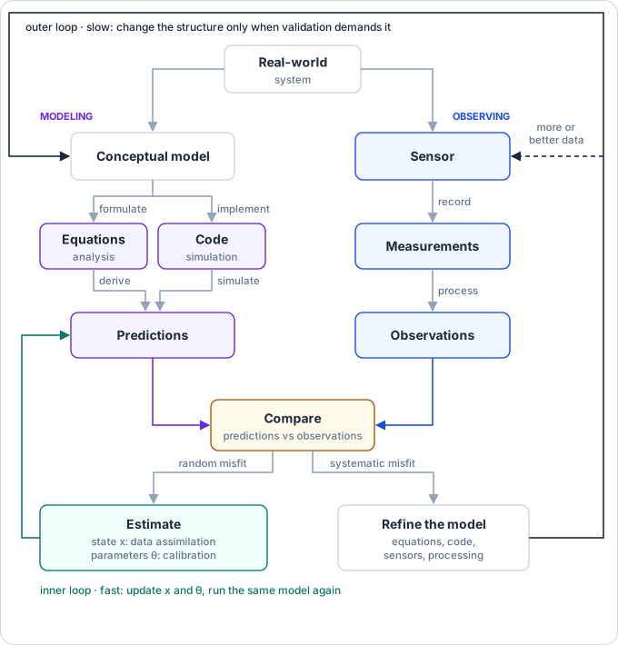
Figure 1:The modeling cycle runs on two parallel tracks and two loops.
The modeling track turns a conceptual model of the real-world system into equations and code that make predictions. The observing track measures the same system with sensors and turns measurements into observations. The tracks meet where predictions are compared with observations, and the misfit decides which loop runs. A random misfit, one the error model explains, runs the fast inner loop: state estimation (data assimilation) updates the state , parameter estimation (calibration) updates the parameters , and the same model runs again. A systematic misfit runs the slow outer loop: the model’s structure changes, or the observing system does (more or better data, better processing).
4.2The L0–L5 data lifecycle (axis 2)
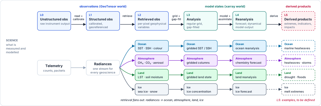
Figure 2:The data lifecycle, science axis.
One stream of radiances fans out into ocean, atmosphere, land and ice at retrieval, and ends in derived products such as extremes (L5, dashed: examples still to be defined). Figure 3 maps the same levels to the tools that handle them.
Table 2:The six levels of the data lifecycle.
| Level | Name | What it holds | Carrier |
|---|---|---|---|
| L0 | Unstructured observations | raw instrument output: telemetry, counts, packets | GeoTensor |
| L1 | Structured observations | calibrated, georeferenced radiances | GeoTensor |
| L2 | Retrieved observations | per-pixel geophysical variables, with gaps where retrieval fails | GeoTensor |
| L3 | Analysis | a regular, gap-filled grid: the “world right now” | xarray |
| L4 | Reanalysis and forecast | dynamical model output: data-constrained, fused or projected | xarray |
| L5 | Derived products | extremes, indicators and impacts computed from L4 | xarray |
Table 2 names the six levels.
The science axis runs left to right. Until retrieval it is one stream, as the same L1 radiances feed every geoscience. Retrieval is where it fans out into ocean, atmosphere, land and ice variables, and each domain then carries its own analysis and reanalysis or forecast. L5 holds the products derived from those states, such as extremes (marine heatwaves, droughts, storms) or impact indicators. Which products belong in L5 is still an open question.
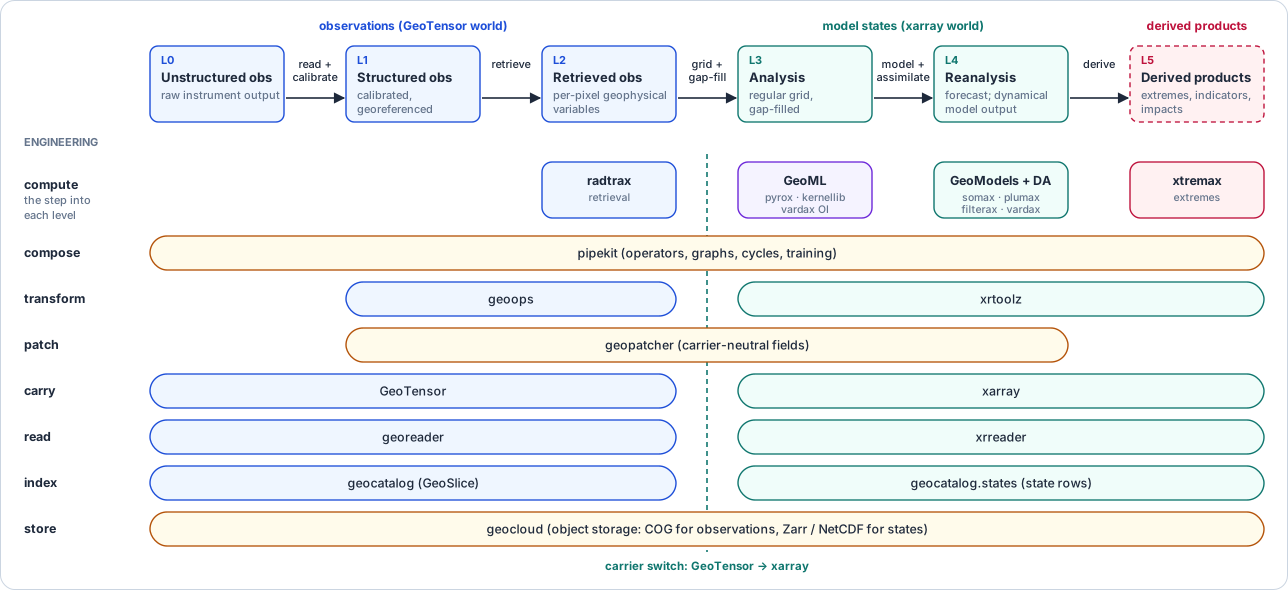
Figure 3:The data lifecycle, engineering axis.
The top row names what performs each step; the rows below map every level to the tool that composes, transforms, patches, carries, reads, indexes and stores it, switching carrier from GeoTensor to xarray between L2 and L3.
The engineering axis runs top to bottom, from computing a level down to storing it, and it maps every level to the GeoStack tool that handles it.
Compute: what performs the step into each level. radtrax retrieves (L1 → L2). GeoML grids and gap-fills (L2 → L3: pyrox, kernellib, the optimal interpolation of vardax). GeoModels with data assimilation model and assimilate (L3 → L4: somax and plumax with filterax and vardax), which is the inner loop of Figure 1. Lastly, xtremax derives extremes (L4 → L5).
Compose:
pipekitwires every level into operator graphs, cycles and training loops, whatever the carrier.
The rows below split where the carrier changes:
Observations (L0 to L2):
georeaderreads them into a GeoTensor,geocatalogindexes them as GeoSlices andgeotoolztransforms them.Model states and derived products (L3 to L5):
xrreaderreads them into xarray,geocatalog.statesindexes them in the same catalogs as state rows (its state profile), andxrtoolztransforms and verifies them.Both carriers:
geopatcherpatches fields whatever the carrier, andgeocloudstores both on object storage (COG for observations, Zarr or NetCDF for states).
ML enters at every transition.
4.3Two streams converge
The lifecycle is not one chain. A top-down satellite stream and a bottom-up in-situ stream converge between L2 and L3 (Figure 4).
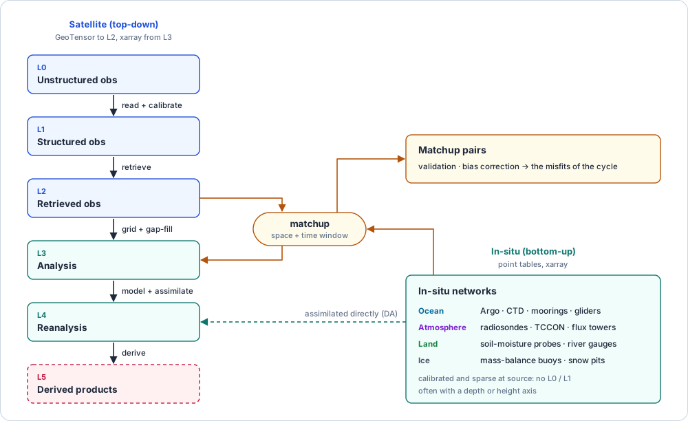
Figure 4:Satellite and in-situ observations converge through matchup.
In-situ networks in every domain join the satellite chain through spatiotemporal matchup between L2 and L3, and enter L4 directly through assimilation. They have no L0 or L1 equivalent. Matchup also yields the pairs that validate and bias-correct the satellite stream: the misfits that drive the loops of Figure 1.
The matchup pattern is canonical and it deserves its own operator family (stage 2 runs it, and where it lives is an open question).
4.4Three layers of transformation
A third lens joins the cycle and the lifecycle, which is what we do to the data on its way into a model (Figure 5).
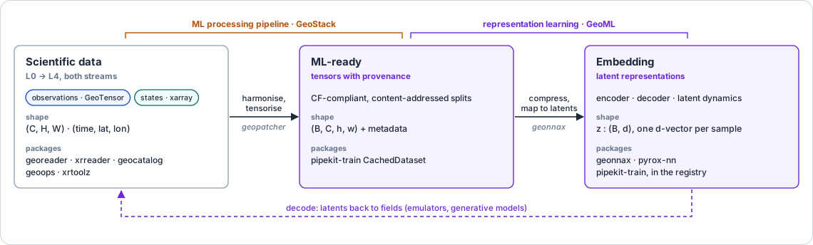
Figure 5:Scientific data, ML-ready data, embeddings, and who owns each.
The first step is data engineering (GeoStack), the second representation learning (GeoML). The middle layer is the handoff that makes training reproducible: cached, CF-compliant tensors with content-addressed splits. Decoders run the chain backwards, which is what emulators and generative models do.
4.5The six-step cycle (axis 3)
The six-step cycle is the journey from research to production (Figure 6). Every domain library follows this cycle implicitly, and the framework makes it explicit and composable.
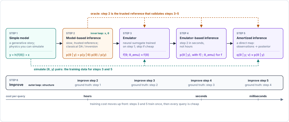
Figure 6:From a simple model to amortized inference, with one shared improve step.
Step 2, the classical method, is the oracle that validates steps 3–5; it is the inner loop of Figure 1. Step 1 also simulates the (θ, y) pairs that train the emulator and the amortized map. Step 6 is shared: any of steps 2–5 can be improved, using the previous step as ground truth, and changing the structure is the outer loop. Moving right, the cost of each query falls from hours to milliseconds because the training cost is paid once, up front.
In symbols, let be the quantity we want (an emission rate, a model state), the physical forward model, the observation operator, the observations and their error, with covariance . In the six-step cycle (and in its figures), stands for whatever we infer, so it covers both the state and the parameters of Figure 1. Step 1 is the generative story:
where the error is Gaussian,
Step 2 inverts it with classical, model-based inference. Bayes’ rule with a prior defines the target:
Computing (3) is only exact in tractable cases, such as a linear-Gaussian model solved with the Kalman filter or a GP. The usual step-2 methods (a finite-ensemble EnKF, 3D- or 4D-Var) approximate it, and slowly. So step 2 is the oracle because it is the most trusted reference we have, and not because it is exact.
Step 3 trains an emulator with weights on step-1 simulations by (4), and step 4 reruns step 2 with in place of :
Step 5 skips the inversion. It trains a conditional density with weights , which maps observations straight to an approximate posterior, on pairs drawn from the generative model (1), by (5):
so that the trained density approximates the posterior,
Table 3 says where each step lives in the stack. There are two structural commitments which fall out of the cycle:
Classical methods (filterax, vardax, pyrox) are not legacy code waiting to be replaced by neural emulators. They become reference generators that validate steps 3 to 5. So the classical path stays alive, promoted to oracle.
Writing a benchmark contract (carriers, references, metrics, splits, baselines, expected failure modes) is formalising what you understand about the problem. Every transition between steps is a benchmarkable contract.
Table 3:Where each step lives in the stack.
| Step | Lives in |
|---|---|
| 1 · Simple model | GeoModels (somax, plumax, radtrax) |
| 2 · Model-based inference | pipekit-cycle.DACycle with classical analysis steps |
| 3 · Emulator | pipekit-train.SimulationDataset, registered in pipekit-experiment.ModelRegistry |
| 4 · Emulator-based inference | pipekit-cycle.DACycle with NeuralForward |
| 5 · Amortized inference | pipekit-train with gauss_flows or pyrox |
| 6 · Improve | pipekit-evaluate.Benchmark reruns, compared row by row, with lineage in pipekit-experiment |
4.6How the axes relate
The axes form a cube of operations. At any point you are somewhere on the modeling cycle (research stage), somewhere on the lifecycle (data maturity) and somewhere on the six-step cycle (production maturity). Figure 7 crosses the lifecycle transitions with the steps.
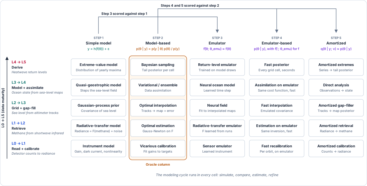
Figure 7:Every lifecycle step crossed with every six-step stage is a concrete method.
Each row follows one running example from a simple model to an amortized map: radiance from detector counts, methane from shortwave infrared, sea level from altimeter tracks, the ocean state from sea-level maps, and heatwave return levels.
Every cell is a benchmarkable artifact, scored against the earlier step that computes the same thing (an emulator against the simulator it replaces, and emulator-based and amortized inference against the posterior of the step-2 oracle). The benchmark ladder of pipekit-evaluate ships this rule (Report 17). The whole lifecycle is a nested set of six-step cycles, each gated by benchmarks. This is what makes the framework improvable in practice, since improving a cell re-runs its downstream column, the lineage is content-addressed, and nothing is opaque.
5The big picture stack
We show the stack at two zoom levels: the layers first, then the packages inside GeoStack.
5.1Four layers
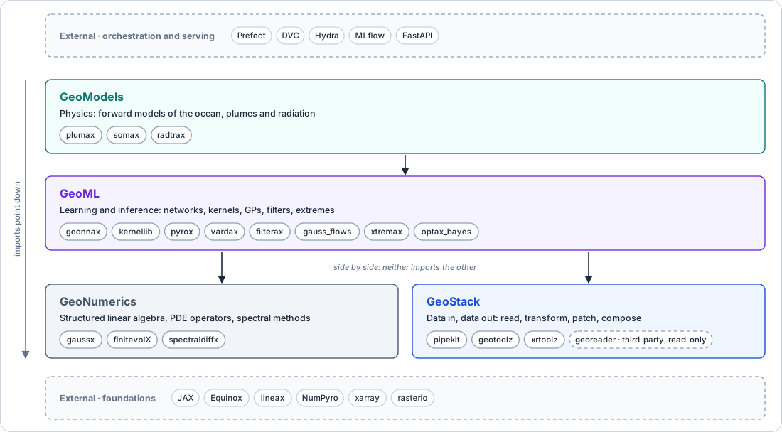
Figure 8:The stack in four layers.
Each layer has one job: GeoStack moves data in and out, GeoNumerics does
structured numerics, GeoML learns and infers, GeoModels simulates physics.
Imports point down, and GeoStack and GeoNumerics never import each other
(Figure 10 and tests/test_dependency_graph.py check it).
Dashed rows are external; georeader belongs to GeoStack but is
spaceml-org’s, read here and never written.
5.2GeoStack, zoomed in
Most of the current work happens in the GeoStack layer (Figure 9).
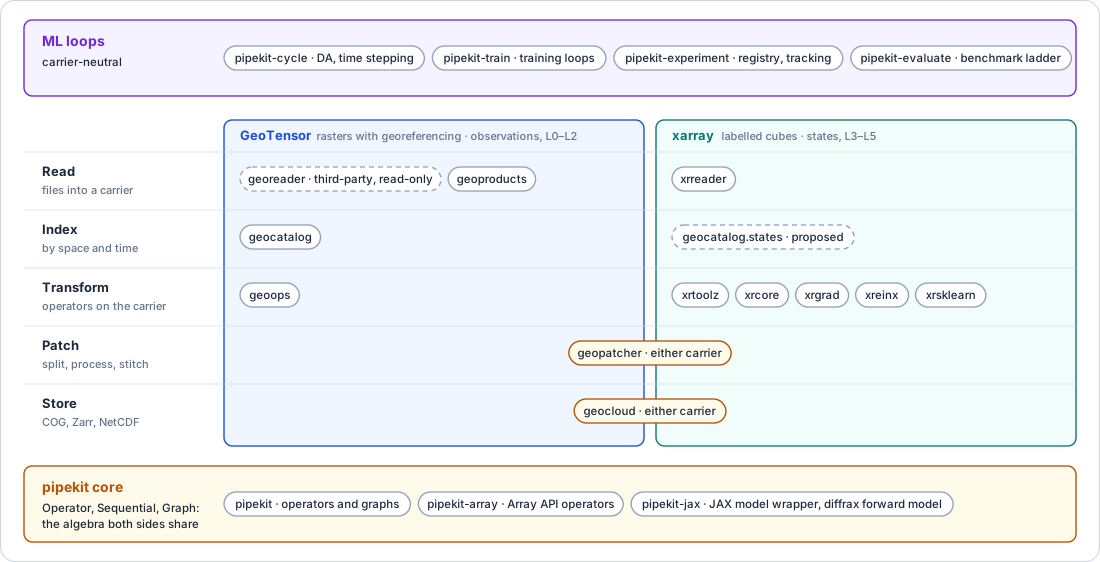
Figure 9:One pipekit core, two carriers, the same jobs on both.
Row by row, the GeoTensor side and the xarray side do the same job on a different carrier; patching and storage serve both. The ML loops on top never see which carrier they run on.
5.3The dependency graph
Figure 10 shows which repositories import which.
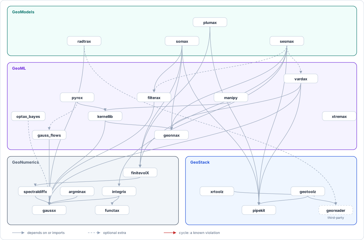
Figure 10:How the repositories import each other.
Drawn from the generated graph on the
dependency-graph page, which
tests/test_dependency_graph.py keeps current; that page has the
package-level detail and the table of known violations. Solid edges are
dependencies or imports, dashed edges optional extras, and red edges a cycle.
5.4Ownership rules
A package only imports from the layers below it, so there are no circular dependencies. geotoolz and xrtoolz re-export the common framework symbols, so user code usually imports a single package. Each of the three stacks of the decision has its own rules. The GeoStack rules (pipekit and its packages, geocatalog, geopatcher, geotoolz and xrtoolz) are in Report 16, and the GeoModels rules (somax, plumax, radtrax, on top of the GeoNumerics layer) are on the package boundaries page. The GeoML rules are only stated here: the JAX libraries touch pipekit only through an optional adapter module, and never in their core.
gaussx owns structured linear algebra and Gaussian primitives. It imports no GeoStack package.
geonnax owns basis functions, neural layers and coordinate transforms. somax and the other models compose them and never reimplement them.
kernellib owns covariance kernels and tapers. It imports no inference library.
optax_bayes owns the Bayesian learning rule as optax transforms. It imports no model library.
spectraldiffx and finitevolx own discretisations (spectral and finite-volume operators, no physics).
pyrox owns GP and Bayesian NN building blocks for NumPyro. Its pipekit surface (
KrigingOperator) only lives inpyrox.adapters.pipekit.filterax owns ensemble Kalman methods and vardax owns 3D/4D-Var. Each one only exposes an
AnalysisStepthroughadapters/pipekit.py.gauss_flows owns Gaussianization and normalizing flows, and xtremax owns extreme-value and point-process models. Neither imports pipekit outside an adapter.
6Walkthrough: methane attribution
This is the canonical example, a complete pipeline from satellite scenes to source emission estimates, with ML at several stages.
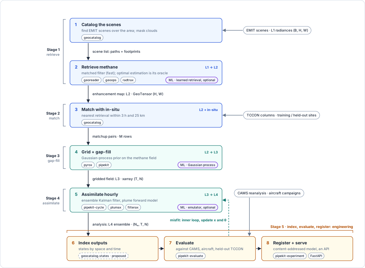
Figure 11:Eight steps from cataloguing scenes to serving estimates.
Stages 1–4 are the science, stage 5 the engineering around it. Each arrow names what flows to the next step; the dashed arrow is the inner loop of Figure 1, the misfit that updates the state and parameters.
For the data, we use EMIT imaging-spectrometer scenes (L1 radiances) over an area of interest, TCCON column measurements as in-situ truth, and CAMS reanalysis and aircraft campaigns as evaluation references. The dimensions we use below are spectral bands, pixels per scene (H × W in the code sketches), observations, grid cells, ensemble members (N_e in the code) and hourly steps.
The eight steps of Figure 11 group into five stages. Each stage states the problem it solves before the code does, and stages 3 and 4 have closed-form special cases which double as test oracles (Table 6).
6.1Stage 1 · Retrieve methane (steps 1–2: geocatalog → georeader → geotoolz)
TL;DR. Find every EMIT scene over the area, mask clouds, and turn each pixel’s spectrum into a methane enhancement.
Problem. For pixel , is its radiance spectrum, is the scene-background mean, is the background covariance and is the methane target signature (unit absorption times ). The matched-filter enhancement estimate is the least-squares amplitude of in the whitened residual:
The matched filter (7) is the fast classical enhancement estimate, and its derivation is in radtrax · 1. The full-physics retrieval (optimal estimation on a radiative-transfer model) is step 2 of the six-step cycle for the L1→L2 cell (Figure 7). A learned retrieval takes the same slot in the pipeline, and optimal estimation stays as its oracle.
6.2Stage 2 · Match with in-situ (step 3: geocatalog matchup)
TL;DR. Pair each TCCON measurement with the one satellite retrieval nearest to it in space and time; measurements with nothing nearby are dropped.
Problem. In-situ observation sits at location and time , satellite retrieval sits at and , and is the great-circle distance. The candidates for are the retrievals inside both tolerances, (8):
If is empty, then has no matchup. Otherwise keeps the single candidate with the smallest scaled distance (9), so no TCCON record is counted twice:
Ties go to the earlier retrieval and then to the smaller catalog index, so the selection is deterministic.
The pairs serve two jobs, so we split TCCON once, by station, before anything is fitted. The pairs from the training sites are the (label, feature) data which a learned retrieval trains on, whereas the pairs from the held-out sites validate stage 1 and are the only TCCON references we use in stage 5. No site appears in both, so the held-out scores never include a label the model saw. How much of the disagreement between the pairs is representativeness error is an open question.
6.3Stage 3 · Grid and gap-fill (step 4: pyrox through pipekit)
TL;DR. Turn scattered retrievals into a regular map with an uncertainty for every grid cell.
Problem. are the L2 retrievals, is their noise variance and is a Matérn-5/2 kernel with a 50 km length scale. is between the observation locations , is between the grid cells and the observation locations (with ), and is between the grid cells. The GP posterior mean and variance on the grid are:
Kriging is the oracle for the L2→L3 cell, and DINEOF and neural gap-fillers are judged against it. Stage 4 assimilates this map, with as its observation and as its observation-error covariance.
6.4Stage 4 · Assimilate hourly (step 5: pipekit-cycle → plumax → filterax)
TL;DR. Step a transport model forward each hour and pull it towards the observations.
Problem. is the methane state at hour , is one plumax transport step of 3,600 s, is the column observation operator, is the stage-3 map for hour , and is the observation-error covariance (here from the stage-3 kriging). The background covariance is estimated from the members. Each cycle forecasts every member by (12):
and then updates each member against its own perturbed copy of the observations (the stochastic EnKF), with drawn independently per member:
where the gain is
The perturbations matter, because if we update every member with the same unperturbed , the anomalies shrink by and the analysis ensemble is too narrow, which would bias the CRPS in stage 5. is inflated by 1.05 and localised with a Gaspari–Cohn taper. The localisation trades exactness for removing spurious long-range correlations, and the perturbations make the estimate random. However, they are drawn from one key seeded from the config of the run, so a rerun reproduces them (gate G1). A square-root (ETKF) variant replaces the perturbations with a deterministic anomaly transform. With a linear and , no inflation and no localisation, its analysis mean equals the Kalman update applied to the sample mean and covariance of the ensemble itself, which is gate D2.
6.5Stage 5 · Index, evaluate, register (steps 6–8: geocatalog.states → pipekit-evaluate → pipekit-experiment)
TL;DR. Store every analysis, score it against three independent references, and attach the score to the model that made it.
Problem. For a forecast distribution with CDF , a reference value , and independent draws from , the continuous ranked probability score is given below. Lower is better, and with one member it reduces to the absolute error. Mass closure checks that the total methane is conserved to within 1 %.
The same pipeline, written as YAML, becomes the regulatory artifact (Report 9, use case 9). The same operators run in a notebook (case 1), an ETL job (case 2), a FastAPI endpoint (case 5) or a Fused UDF (the Fused integration design).
7Per-layer briefs
Here we give a compact summary per package, by layer (Figure 8). Where a report or a GeoModels page covers a package, the brief is a link to it.
The JAX ecosystem: JAX, Equinox, lineax, optax, diffrax, NumPyro and matfree.
The xarray ecosystem: DataArray, Dataset and DataTree, plus rioxarray, xvec, cf-xarray, regionmask, xskillscore, dask and intake.
georeader (third-party, spaceml-org’s, and read-only here) owns GeoTensor, the raster carrier, and the reader infrastructure (RasterioReader, AsyncGeoTIFFReader). Everything raster-shaped builds on it.
| Package | What it does | Read |
|---|---|---|
pipekit | The operator framework: fourteen groups (A–N) | Report 2, Report 1 |
pipekit-array | Array-API operators | Report 3 |
pipekit-jax | A model wrapper and a diffrax forward model; the operator layer is proposed | Report 5 |
pipekit-cycle | Time stepping and DA cycles | Report 10 |
pipekit-train | Training pipelines | Report 11 |
pipekit-experiment | Model registry and tracking | Report 12 |
pipekit-evaluate | The benchmark ladder | Report 14, Report 15, Report 17 |
geotoolz | GeoTensor operators for remote sensing | Report 3 |
geocatalog (ships as geotoolz-catalog) | Find, index, join and load files | Report 6 |
geopatcher (ships as geotoolz-patcher) | Split, process and stitch patches | Report 7 |
geocatalog.states (proposed state profile) | A catalog for model states | Report 13 |
xrtoolz | xarray operators for ocean, atmosphere and reanalysis | Report 3 |
geotoolz and xrtoolz share the same pipekit operator algebra, and only the carrier differs.
| Package | What it does |
|---|---|
gaussx | Structured linear algebra, Gaussian primitives, exponential family; wraps lineax and matfree |
spectraldiffx | Pseudospectral differentiation, filters, PDE solvers |
finitevolx | Arakawa C-grid finite-volume operators |
This layer is pure math with no domain knowledge, and all of it is eqx.Module-based, jittable and JAX-traceable. See the gaussx example.
| Package | What it does |
|---|---|
geonnax | Basis functions, neural layers and coordinate transforms (lonlat_to_cartesian3d) |
kernellib | Covariance kernels and scalable kernel methods |
pyrox | GP and Bayesian deep-learning building blocks for NumPyro models |
vardax | Learnable variational DA (3D- and 4D-Var) |
filterax | Differentiable ensemble Kalman methods |
gauss_flows | Rotation-based Gaussianization and normalizing flows |
xtremax | Extreme-value and point-process models; computes the L5 extremes |
optax_bayes | The Bayesian learning rule as optax gradient transformations |
The adapter of each library (*.adapters.pipekit) makes it composable into pipekit pipelines, whereas the core never imports pipekit. See the filterax example.
| Package | What it does | Read |
|---|---|---|
somax | Ocean and atmosphere model zoo | — |
plumax | Atmospheric plume transport | plumax · 1, package boundaries |
radtrax | Differentiable radiative transfer (formerly rtmx) | radtrax · 3 |
The forward models each ship a thin adapters/pipekit.py which exposes the operator surface (ForwardModel, ObservationOperator, …) without touching the algorithmic core.
8Key code patterns
Each pattern has runnable-looking code on the overview examples page.
How an operator like PercentileClip is written.
Sequential, the pipe syntax, and DAGs with Graph.
Build, query and match a geocatalog.
Geometry × sampler × window × aggregation.
Protocol-satisfying parts composed into a DACycle.
Replace a classical forward model with a neural one.
Multi-track evaluation as a content-addressed artifact.
A pre-registerable, content-addressed benchmark.
Freeze a pipeline for a regulatory cold rerun.
9Open questions
None of these block the work, but all of them deserve some thought before we commit to a decision.
Raised by the design review
What
InferenceArtifactstill needs for a cold rerun. The shippedInferenceArtifactalready saves and loads the YAML of a pipeline, its pinned model hashes, the lockfile and metadata. Arerunwhich rebuilds the pipeline and pulls its frozen inputs is proposed. What is still open is 1) whether that rerun resolves inputs from the pinned catalog URIs and SHA-256 digests alone, without cloud credentials, and 2) how aBenchmark(not yet serialisable) is frozen next to it.
Resolved elsewhere
Serialising a
Graph. Emitting a built pipeline as YAML that loads back is proposal A of Report 9. Until it lands, gate A1 only covers YAML-safe operators.A per-step observation error. An
obs_err_sourceis proposed in Report 10, workstream B.Two evaluation APIs. Report 15, workstream D builds the contract and the tracks on the shipped
Benchmarkcube (from_contract, several references per run), with no separateMultiTrackEvaluation.Where
xrreaderstops andgeoreaderstarts. A mission reader lives with its output carrier (Report 16, workstream E).Which stack somax and spectraldiffx belong to. Rule 5 of the package boundaries puts somax in GeoModels, and spectraldiffx and finitevolx in GeoNumerics. methanex is still unplaced.
Sequencing
When does pipekit-jax’s operator layer land? pipekit-jax 0.0.2 has shipped as a model wrapper and a diffrax forward model (Report 5), whereas the operator layer is still proposed. The six-step cycle gives it a concrete driver, since differentiable step-3 emulators make step 4 (gradient-based inverse problems) tractable at scale. It stays open until such a project appears.
Which in-situ catalog backend comes first? The scoping proposal behind Report 6 leaned to Argo (via argopy), but ICOADS, SOCAT and the World Ocean Database matter for other domains. Realistically, we can do one per quarter, driven by projects.
Design
The Slice Protocol refactor.
GeoSliceis the only slice type today. AddingProfileSliceandTrajectorySliceis the right structural move, but it is two weeks of work which ripples across geocatalog, geotoolz, xrtoolz and pipekit-train. So it is better done before more code commits toGeoSlice.Where matchup lives.
geocatalog.queries.matchup()is the framework function, with carrier-specific helpers in xrtoolz and geotoolz. Does matchup need its own catalog type? Probably, but it is not scoped yet.Backend choice in pipekit-train. Equinox + Optax and the Bayesian backends ship, whereas Lightning and Keras 3 are scaffolds (Report 11). The intended split is Lightning for PyTorch models, Equinox + Optax for JAX-traceable pipelines and Keras 3 for multi-backend. This is worth stating per use case.
Operational
Monorepo or polyrepo? A monorepo for the framework and infrastructure (uv workspaces), whereas the JAX-native algorithm and domain libraries stay in their own repositories and ship adapter modules.
One documentation site or many? One site for the monorepo packages, separate sites for the algorithm libraries, and one research journal which cuts across everything.
CI per package or per monorepo? Per-package CI inside the monorepo, plus one weekly integration matrix which pins every package to HEAD. Releases go by git tag (
geocatalog-v0.2.0).
Scientific
Matchup UQ.
MatchupPair.representativeness_uncertaintyis easy to declare and hard to compute, so v0.1 ships a placeholder.Cascading uncertainty. A five-stage emission chain accumulates uncertainty across stages. Predicting that honestly is still open research.
Probabilistic event detection. “A plume happened” is binary, whereas “a 73 % chance a plume happened” is much harder, and the current event metrics assume the binary case.
Sustainability
Solo maintenance. About twenty packages is a lot, even with monorepo discipline. So scope discipline is the operating constraint: each phase delivers standalone value, and no layer needs the full stack to exist.
Community adoption. If oceanbench adopts the benchmark contracts of pipekit-evaluate, the framework is validated, and if not, it stays personal infrastructure. When to start reaching out is still open.
10A plan
Each phase produces packages which are useful on their own (Table 4).
Table 4:Phases at a glance.
| Phase | Scope | Status | Time |
|---|---|---|---|
| 1 | GeoNumerics: gaussx (v0.0.6), spectraldiffx, finitevolx | gaussx done; the rest drafts | ongoing |
| 2 | GeoML: geonnax, kernellib, optax_bayes, pyrox, filterax, vardax, gauss_flows, xtremax | in progress | each at its own pace |
| 3 | GeoModels: somax, plumax, radtrax | some done | project-driven |
| 4 | Pipeline framework | current focus | ~3–4 months |
| 5 | Evaluation, benchmarks and cycle discipline | next | ~2 months |
| 6 | Deferred items, each with a trigger | when projects demand | — |
| 7 | Polish and community | open-ended | — |
10.1Phases 4 and 5, month by month
pipekit 0.0.2: framework core, fourteen groups and state primitives (shipped; Report 2)
pipekit-array 0.0.2: Array API operators (shipped, phase A of four; Report 3)
the pipekit-ecosystem monorepo with uv workspaces
Gate: A1 config round-trip (Table 6).
geocatalog v0.1: InMemory and DuckDB backends, basic queries
geopatcher v0.1: the four-axis framework and five Field adapters
geotoolz and xrtoolz refactored onto the new framework
Gates: B1 backend parity, C1 patch identity.
geocatalog’s state profile (
geocatalog.states) and xrtoolz forecast alignmentpipekit-cycle 0.0.2:
Cycle,DACycleand the protocols (shipped; Report 10)adapter modules in filterax, vardax and plumax
Gates: B2 state rows, D1 kriging oracle, D2 Kalman oracle.
pipekit-train 0.0.2 ships Equinox + Optax and the Bayesian backends, whereas Lightning and Keras 3 are scaffolds (Report 11)
pipekit-experiment 0.0.2 ships the registry and the tracker protocol, and the MLflow and W&B trackers are planned (Report 12)
integration testing across all packages
Gate: E1 registry round-trip.
After Phase 4: the L0 to L4 inference loop is structurally complete. ML training and serving still need work, but the pipelines exist.
pipekit-evaluate v0.1: framework, cheap metrics,
EvaluationReportleakage-aware splits: block, platform and causal splits of catalog rows in geocatalog, and the window guard in time units in pipekit-train
standard baselines in xrtoolz: persistence, climatology, OI
lineage in pipekit-experiment’s content hash, with a dependents query (the six-step cycle’s lineage, Report 17)
Gate: F1 metric identities.
particle tracking (
xrtoolz.lagrangian) and event detection (xrtoolz.events)BenchmarkContractwith transition cells and an oracle strength (Report 17)several references per run in the benchmark runner (Report 15)
the first worked cycle (likely methane L1→L2 retrieval, steps 1 to 5)
the first worked benchmark (SSH, from the benchmarks gallery)
Gate: G1 end to end.
After Phase 5: evaluation is first-class, benchmarks are content-addressed contracts, and the six-step cycle is tractable end to end.
10.2Deferred until a project needs it
Table 5 lists what waits for a project, and what pulls it in.
Table 5:Phase 6: what is deferred, and what triggers it.
| Item | Trigger |
|---|---|
| pipekit-jax’s operator layer (operators as PyTrees; 0.0.2 ships only a model wrapper and a diffrax forward model, Report 5) | the first project needing differentiable retrievals at scale or JIT-compiled inference |
Deployment adapters (pipekit_ops.deploy.fused, .litserve, .modal) | the first deployment beyond hand-shimming |
Slice Protocol refactor (ProfileSlice, TrajectorySlice) | the first project needing first-class in-situ catalogs (likely the BGC benchmark) |
| More in-situ backends (Argo, ICOADS, SOCAT, …) | one per quarter, project-driven |
Phase 7 covers the documentation site, a research journal, the first external benchmark adoption (OceanBench, WeatherBench-Ocean?) and capstone tutorials per domain.
10.3Gates
A month is done when its gates pass, and not when its packages exist (Figure 12). Every pass condition is a number or a closed form, and several of them reuse the closed-form stages of the walkthrough as oracles (Table 6).

Figure 12:The framework ships first; every month closes on its gates.
Phases 1–3, one per lower layer, run alongside and meet the chain twice: the DA adapters land in month 3 and the GeoML models are trained in month 4. Phases 6 and 7 wait for projects to pull them.
Table 6:Gates: what must pass before each month closes.
| Gate | Workstream | Passes when |
|---|---|---|
| A1 Config round-trip | A | For every shipped operator not marked forbid_in_yaml, loads(dumps(op)) has the same config hash and returns the same output on a fixed input; once the topology serialiser lands, the same holds for a Graph (as Report 9’s A1) |
| B1 Backend parity | B | The InMemory and DuckDB geocatalog backends return the identical slice set for the same bbox and time query |
| B2 State rows | B | A cycle’s ensemble history, written as one file per run and member and indexed with build_state_catalog, loads back with load_states with no run dropped and equal to the history to 0 (Report 13, gates A2 and B1) |
| C1 Patch identity | C | An identity model through patch → stitch with Hann-window overlap-add reproduces the input to 1e-6 in float64, away from scene edges |
| D1 Kriging oracle | D | KrigingOperator’s mean and variance match (10) and (11) to 1e-6 in float64 |
| D2 Kalman oracle | D | With linear and , no inflation and no localisation, the square-root ensemble analysis mean matches the Kalman update computed from the same ensemble’s sample mean and covariance, to 1e-6 in float64 |
| E1 Registry round-trip | E | Loading a stored operator returns one with the same content hash and bitwise-equal outputs |
| F1 Metric identities | F | CRPS (15) with one member equals absolute error exactly; RMSE of a field against itself is 0 |
| G1 End to end | all | Stages 1–5 of the walkthrough run from one YAML file. A cold rerun of the frozen inference artifact reproduces the analysis history’s hash, and rerunning the frozen benchmark (its task, estimators, scorers and pinned TCCON references) on that history reproduces the report’s hash |
10.4Risks
The schedule slips. Six months for Phases 4 and 5 is optimistic for one person, and eight to twelve is realistic. Fallback: every month ships a usable package, so nothing depends on the whole plan finishing.
Phase 6 is needed early. A project may need pipekit-jax or in-situ catalogs before the framework is ready. Fallback: we wrap jitted functions in pipekit-jax’s
JaxModelOpuntil the full backend lands, and we jump phases, since the sequence is a default and not a contract.The Slice refactor ripples late. The longer
GeoSlicestays concrete, the more code binds to it. Fallback: we introduce aSliceprotocol in month 2 withGeoSliceas its only implementation, and add profile and trajectory slices later.pipekit-train becomes three half-backends. Equal status for Lightning, Equinox and Keras 3 triples the maintenance. Fallback: one default backend per use case, and the others are community-supported.
Nobody else adopts it. Adoption takes years. Fallback: GeoBench is the first consumer, so the substrate earns its keep without outside users.
11Where to read next
11.1How the pages are written
Each page checks a design, a scoping report or a source note against the code pinned in references/, and the code takes precedence. A Differs box marks each place where the code (or a check the page runs) disagrees with the design. The gaps that matter become workstreams with proposals, and the rest go to open questions or upcoming work. Every number on a page comes from a notebook which asserts it. Pseudocode follows one convention: 1) a shapes header names the dimensions, 2) the equation sits in a comment above the line that computes it, 3) shapes go on the right, and 4) every call into the stack carries a status marker (markers).
11.2The pages
We suggest you start with the capability index and the overview examples, and then read by question.
Across the stack
Report 9: twenty use cases mapped onto the libraries as they ship.
Report 16: the geo data stack, the ownership rules and the realignment plan across 18 distributions.
pipekit
Report 1: the toolz lineage, and why pipekit’s operators are classes; now pipekit’s Background page.
Report 2: what pipekit 0.0.2 ships, in fourteen groups (A to N); the tour is now pipekit’s tour of the core, and the planning stays here.
Report 5: jit, vmap and grad through pipelines, and what pipekit-jax ships.
Report 10: pipekit-cycle, time-stepping and data assimilation.
Report 11: pipekit-train, training for emulators and amortized inference.
Report 12: pipekit-experiment, the registry, trackers and reproducibility artifacts.
Report 14: pipekit-evaluate, multidimensional evaluation.
geotoolz and xrtoolz
Report 3: the sister libraries, pipekit-array, geotoolz and xrtoolz.
Report 6: geocatalog, the spatiotemporal index.
Report 7: geopatcher, the four-axis patcher.
Report 13: L3 to L5 indexing, as geocatalog’s state profile.
Benchmarking
Report 15: benchmarks as content-addressed contracts.
Report 17: the six-step cycle as the benchmark ladder, step 2 as oracle.
Benchmarks gallery: eighteen draft benchmark entries in five domains.
GeoModels
Package boundaries: what moves from geotoolz and plumax into plumax and a new radtrax.
radtrax · 1: the Beer–Lambert column retrieval, term by term.
radtrax · 2: the SBMP, MBSP and MBMP family of multi-band retrievals.
radtrax · 3: radtrax’s design and roadmap (formerly rtmx).
plumax · 1: emission rate from first principles, from the plume to the IME.
12In summary
GeoStack is one operator algebra from structured linear algebra to indexed multi-tier data products, which is organised by three orthogonal axes and split into the three stacks of the decision. Classical methods stay as oracles, benchmarks are content-addressed contracts, and differentiability only lives in the JAX packages. The plan is a default sequence which projects will reshape. So pick a page from Where to read next and come back with questions, since no part of the stack requires the rest.
13Glossary
- carrier
- The data structure an operator acts on: NumPy or JAX arrays, a GeoTensor, or an xarray object. pipekit operators are carrier-agnostic.
- GeoTensor
- georeader’s raster carrier: an array with its geotransform and CRS. The carrier for L0 to L2.
- GeoSlice
- geocatalog’s wire format for one spatiotemporal slice of an observation catalog.
- state profile
- geocatalog’s reserved columns for model states (run time, ensemble member, producer hash and parent state) and the loader and queries in
geocatalog.statesthat use them. It replaces the plannedstatecatalogpackage and itsStateSlice. - matchup
- Pairing observations from different sources that coincide in space and time; the operation where the satellite and in-situ streams converge.
- oracle
- The classical method (step 2) used as the trusted reference to validate emulators and amortized predictors.