GeoStack vision: one vocabulary from file to analysis

The same operator runs in a concurrent ETL, a compiled training step and a lazy cube; users choose how much control they take and how it runs, independently. Keras made that choice for training on one backend at a time; GeoStack makes it for whole pipelines, mixing run modes within one run.

1Progressive disclosure¶

A user starts with a packaged pipeline and steps down only as far as the work needs, as in Keras; each stop is built from the one below it.

A horizontal spectrum with four stops. L3, a packaged pipeline with built-in operators, gives standard workflows, fast and easy (emit_plumes.v1.run). L2 plus pipekit, a pipekit graph of built-in operators, gives new workflows from existing components. L2 with your own KernelOps and operators gives new components (SwathToGrid, Detector). L1, primitives on arrays in your own loop, gives anything you want (vmap of matched_filter_score). 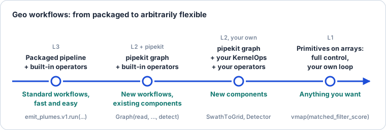— Figure 1:**Four stops, from packaged to arbitrarily flexible.** Each stop is built from the one to its right and hands it back.

The stops come from two independent axes: what each step computes (built-in operators down to primitives) and how steps are put together and run (packaged runners down to your own loop).

Two crossing axes inside an ellipse. Horizontal, computation, from low-level primitives on arrays plus derived geometry to high-level built-in operators. Vertical, orchestration, from your own loop (lax.scan, async I/O) to high-level built-in runners (ETL, train, assimilate) and packaged pipelines. The top right is easy to use; the bottom left is fully flexible. Custom pipekit graphs, KernelOp around your kernel and operator chains such as Mask then NDVI sit in between. 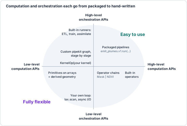— Figure 2:**Computation and orchestration each go from packaged to hand-written.** The four stops are points on these two axes.

Run mode (eager NumPy, compiled JAX, lazy xarray) is a third axis, orthogonal to both: any point on this picture runs in any mode the carrier allows (next section).

2Two axes¶

Control (how much a user writes) and run mode (how it executes) are independent: any level runs in any mode, and the operator row is what all of them share.

Level	eager (NumPy carrier)	compiled (JAX carrier)	lazy (xarray carrier)
L3 pipeline or algorithm	`emit_plumes.v1.run(...)` on one scene	`vardax.geo.assimilate(...)` with its loop under `jit`	an MLD climatology over GLORYS
L2 operator	`ndvi(scene)`	`jax.jit(ndvi)(jscene)`	`ndvi(cube)`, one task per chunk
L1 primitive	`matched_filter_score` on NumPy arrays	`jax.vmap(matched_filter_score)`	the same kernel, called per chunk by `KernelOp`

Read down a column to trade convenience for control; read across a row to change how the same code runs.

3The three levels¶

Every package that computes (geotoolz, finitevolX, esmax, plumax, radtrax, vardax) writes its numerics as primitives on arrays, operators on carriers above them, and algorithms on readable geo types at the top. This is the one definition the other design pages link to.

Level	Takes	Returns	Lives in
L1 primitive	arrays, or an array-only bundle (a NamedTuple or `eqx.Module` of arrays), plus derived numeric geometry	arrays	the lowest package that owns the numerics, in `_src/array.py`
L2 operator	a carrier (`GeoArray`, `DataArray`)	the same carrier family	any package that may import that carrier
L3 algorithm or packaged pipeline	readable geo types (`GeoMap`, `GeoTracks`, `GeoImageSeries`)	readable geo types	the package that runs it (esmax, vardax, plumax)

Derived numeric geometry, never the georeference. Space, time and viewing geometry as arrays: Δx, Δy, cell areas, Δt, sun and view angles, unit vectors on the sphere. A primitive never receives a CRS, a transform object or a pyproj handle.
Operators derive it. KernelOp generates the operator when the only geometry is a dim name (NDVI, the matched filter); an operator is hand-written when it must derive geometry from the carrier.
Algorithms cross the carrier boundary once. They unwrap at entry, call L1 primitives directly inside their loops, and rewrap at exit; they never call L2 operators per step.
A packaged pipeline is a graph of named L2 operators with readable types at its ends, so the four stops below are the three levels plus the graph that composes them.
Exceptions. Geometry operators whose engine is not array code (GDAL rasterize, shapely predicates) have no primitive and are eager only. Reprojection splits: the operator computes source pixel coordinates with pyproj; the primitive is the gather.
Primitives check shapes, not meaning. Units, CRS and grid compatibility are checked at L2 and L3.
Enforced by a test in geostack’s dependency-graph suite: */_src/array.py imports none of geoarray, xarray, pyproj, rasterio, geopandas or shapely.

Where each level sits in every package above GeoStack is on Levels across the stack; where the operator packages sit relative to each other is the tiers.

4Control: four stops, one plume pipeline¶

A user picks how much control to take, as in Keras’s progressive disclosure (Sequential → functional → subclassing). The four stops are the ones in Figure 1.

Stop	You call	You hold	Typing	Who
1. Packaged pipeline (L3)	`plumax.pipelines.emit_plumes.v1.run(...)`	readable geo types	checked on entry and exit	operations, production, benchmarks
2. Graph of operators (L2 + pipekit)	`pipekit.Graph(read=..., matched_filter=..., ...)`	named stages	dims, per stage	analysts building a new workflow
3. Operators (L2)	`SwathToGrid(...)(swath)`, your own `KernelOp`	a carrier with named dims	dims and grids	method developers adding a component
4. Primitives (L1)	`matched_filter_score(x, mu, sigma, t)`	`.data` and derived geometry	shapes	full control: new numerics, your own loop

One running example: methane plumes from one EMIT scene. Each stage needs a different kind of code from a different repo, so every level shows up.

Stage	Computes	L1 primitive (repo)	L2 operator (repo)
read	L1B radiance on the sensor swath, 285 bands	—	`geoproducts.emit.ReadL1B` (geotoolz)
matched filter	α per pixel, μ and Σ per detector column	`matched_filter_score` (radtrax)	`MatchedFilter`, a `KernelOp` (radtrax[geo])
orthorectify	swath → UTM grid at 60 m	`gather_bilinear` (geoops)	`SwathToGrid`: pyproj → source coordinates (geoops)
detect	plume probability per pixel	`PlumeUNet.__call__` (geonnax)	`Detector`, a `JaxOperator` (plumax[geo])
vectorize	mask → polygons	none: GDAL	`geoops.geom.Vectorize`, eager only
the pipeline	all of the above	—	`plumax.pipelines.emit_plumes` (plumax)

The pipeline lives in plumax because it is the lowest package that may import all four: radtrax (GeoModels, tier below), geonnax (GeoML) and geotoolz (GeoStack). The matched filter runs before orthorectification on purpose: its statistics are per detector column, which only exist in sensor geometry.

Stop 1 — L3: a packaged pipeline¶

The user names a scene and gets plumes back; nothing about bands, swaths or models is visible.

# a versioned, packaged pipeline
pipeline: Pipeline = plumax.pipelines.emit_plumes.v1
run: PipelineRun = pipeline.run(scene_id="EMIT_L1B_RAD_001_20260714T081512")

# GeoPoints["variable obs"]: one row per plume (polygon, area, max ΔXCH₄)
plumes: Detections = run.output

Stop 2 — L2 + pipekit: the same pipeline as a graph¶

This is the body of emit_plumes. Every stage is a named, built-in operator; an analyst copies it, reorders or adds stages, and runs it.

def emit_plumes(scene_id: str) -> pipekit.Graph:
    # → GeoSwath["band row col"], 285 bands; lat/lon and sun/view angles as leaves
    read: Operator = geoproducts.emit.ReadL1B(scene_id)

    # t: the unit CH₄ absorption spectrum at EMIT's wavelengths, (C,)
    target: Float[Array, "C"] = radtrax.ch4_unit_spectrum(EMIT_WAVELENGTHS)
    # GeoSwath["band row col"] → GeoSwath["row col"]: α, fitted per detector column
    matched_filter: Operator = radtrax.geo.MatchedFilter(
        target=target, dim="band", fit_per="col"
    )

    # GeoSwath["row col"] → GeoArray["y x"]: the scene's UTM zone at 60 m
    ortho: Operator = geoops.geom.SwathToGrid(crs="utm", resolution=60.0)

    # GeoArray["y x"] → GeoArray["y x"]: plume probability, compiled
    detect: Operator = plumax.geo.Detector.load("plume_unet_v7")

    # p > 0.5 → GeoArray["y x"], bool
    threshold: Operator = geoops.Threshold(0.5)

    # mask → polygons; eager only (GDAL)
    vectorize: Operator = geoops.geom.Vectorize()

    return pipekit.Graph(
        read=read,
        matched_filter=matched_filter,
        ortho=ortho,
        detect=detect,
        threshold=threshold,
        vectorize=vectorize,
    )


graph: pipekit.Graph = emit_plumes("EMIT_L1B_RAD_001_20260714T081512")
plumes: Detections = graph.run()

Stop 3 — L2: operators, one per concern¶

Inside each stage: an operator takes a carrier, derives the geometry its primitive needs, calls the primitive, and rewraps. Three shapes of operator appear here.

# geoops/geom/operators.py — a geometry operator: pyproj here, numerics in L1
class SwathToGrid(Operator):
    backends: tuple[str, ...] = ("numpy", "jax")

    def __init__(self, crs: str, resolution: float) -> None:
        self.crs: str = crs
        self.resolution: float = resolution

    def __call__(self, swath: GeoSwath["row col"]) -> GeoArray["y x"]:
        # the target grid: UTM zone from the swath centre, extent from its footprint
        target: GridSpec = geoarray.target_grid(
            swath, crs=self.crs, resolution=self.resolution
        )
        # derived geometry: fractional source (row, col) of every target pixel (pyproj + KD-tree)
        rows: Float[Array, "H W"]
        cols: Float[Array, "H W"]
        rows, cols = geoarray.swath_source_coords(swath, target)
        # L1: q(y, x) = ∑ᵢ wᵢ s(rᵢ, cᵢ), bilinear
        gridded: Float[Array, "H W"] = gather_bilinear(swath.data, rows, cols)
        return GeoArray.from_grid(gridded, target, dims=("y", "x"))


# radtrax/geo/operators.py — behind radtrax[geo]; a fitted operator built from KernelOps
class MatchedFilter(FittableOperator):
    def fit(self, swath: GeoSwath["band row col"]) -> "MatchedFilter":
        # μ(col) and Σ(col) over the rows of each column: "(r,c)->(c),(c,d)", Σ on
        # (band, band2); the kernel takes one column, so it is vectorized over col
        stats: KernelOp = KernelOp(
            background_stats,
            KernelSpec("(r,c)->(c),(c,d)", vectorize=True),
            core={"r": "row", "c": "band", "d": "band2"},
        )
        # row is consumed, so the outputs are no longer swaths: plain named arrays
        mu: DimArray["col band"]
        sigma: DimArray["col band band2"]
        mu, sigma = stats(swath)
        return self.with_fitted(mu=mu, sigma=sigma)

    def __call__(self, swath: GeoSwath["band row col"]) -> GeoSwath["row col"]:
        # one column at a time: consumes rows and bands, vectorized over col; Σ's
        # second axis is band2, and the kernel's "C C" hint checks |band| = |band2|;
        # t is the same for every column, so it is a parameter, not mapped
        score: KernelOp = KernelOp(
            matched_filter_score,
            KernelSpec("(r,c),(c),(c,d)->(r)", vectorize=True),
            core={"r": "row", "c": "band", "d": "band2"},
            t=self.target,
        )
        return score(swath, self.mu, self.sigma)


# plumax/geo/detector.py — behind plumax[geo]; geonnax's network, carrier handling here
class Detector(JaxOperator):
    net: PlumeUNet  # an eqx.Module from geonnax; weights are leaves
    patch: int = eqx.field(static=True, default=256)

    def __call__(self, alpha: GeoArray["y x"]) -> GeoArray["y x"]:
        # 256 × 256 patches with 32-pixel overlap: (P, 256, 256), transforms (P, 6)
        patches: GeoArray["patch y x"] = geopatcher.split(
            alpha, size=self.patch, overlap=32
        )
        # one input channel per patch
        x: Float[Array, "P 1 H W"] = einx.rearrange("p h w -> p 1 h w", patches.data)
        # L1 under vmap: logits = f_θ(x) per patch
        net_batched: Callable = jax.vmap(self.net)
        logits: Float[Array, "P H W"] = net_batched(x)
        # p = σ(logits)
        prob: Float[Array, "P H W"] = jax.nn.sigmoid(logits)
        # stitch back onto alpha's grid, averaging the overlaps
        prob_patches: GeoArray["patch y x"] = patches.rewrap(prob, dims=patches.dims)
        return geopatcher.stitch(prob_patches, like=alpha)

The three shapes: a geometry operator that derives index arrays with pyproj (SwathToGrid), a fitted operator made of KernelOps (MatchedFilter), and a JAX operator around a network (Detector). Each lives in the package that may import both its carrier and its primitive.

Stop 4 — L1: primitives, arrays only¶

No carrier, no CRS: arrays in, arrays out, each in its owner’s _src/array.py.

# radtrax/_src/array.py — one detector column: R rows, C bands
def matched_filter_score(
    x: Float[Array, "R C"],
    mu: Float[Array, "C"],
    sigma: Float[Array, "C C"],
    t: Float[Array, "C"],
) -> Float[Array, "R"]:
    # x̃ᵣ = xᵣ − μ
    xc: Float[Array, "R C"] = einx.subtract("r c, c", x, mu)
    # w = Σ⁻¹t, solved, never inverted
    cov: lx.MatrixLinearOperator = lx.MatrixLinearOperator(
        sigma, lx.positive_semidefinite_tag
    )
    w: Float[Array, "C"] = lx.linear_solve(cov, t).value
    # αᵣ = x̃ᵣᵀw / tᵀw
    num: Float[Array, "R"] = einx.dot("r c, c -> r", xc, w)
    norm: Float[Array, ""] = einx.dot("c, c ->", t, w)
    return num / norm


# geoops/geom/_src/array.py — bilinear gather at fractional source coordinates
def gather_bilinear(
    s: Float[Array, "R C"], rows: Float[Array, "H W"], cols: Float[Array, "H W"]
) -> Float[Array, "H W"]:
    xp: ModuleType = array_namespace(s)  # numpy or jax.numpy
    n_rows: int = s.shape[0]
    n_cols: int = s.shape[1]
    # inside the source: 0 ≤ r ≤ R − 1 and 0 ≤ c ≤ C − 1; outside gives NaN, never an index error
    inside_r: Bool[Array, "H W"] = (rows >= 0) & (rows <= n_rows - 1)
    inside_c: Bool[Array, "H W"] = (cols >= 0) & (cols <= n_cols - 1)
    inside: Bool[Array, "H W"] = inside_r & inside_c
    # r₀ = ⌊r⌋ clipped to [0, R − 2], c₀ likewise, so r₀ + 1 and c₀ + 1 are in range;
    # a point on the last row gets r₀ = R − 2, δr = 1, and exactly the last row's value
    r_floor: Float[Array, "H W"] = xp.floor(rows)
    c_floor: Float[Array, "H W"] = xp.floor(cols)
    r0: Int[Array, "H W"] = xp.clip(r_floor, 0, n_rows - 2).astype(int)
    c0: Int[Array, "H W"] = xp.clip(c_floor, 0, n_cols - 2).astype(int)
    # δr = r − r₀, δc = c − c₀
    dr: Float[Array, "H W"] = rows - r0
    dc: Float[Array, "H W"] = cols - c0
    # the four neighbours s₀₀, s₀₁, s₁₀, s₁₁
    s00: Float[Array, "H W"] = s[r0, c0]
    s01: Float[Array, "H W"] = s[r0, c0 + 1]
    s10: Float[Array, "H W"] = s[r0 + 1, c0]
    s11: Float[Array, "H W"] = s[r0 + 1, c0 + 1]
    # q = (1−δr)(1−δc) s₀₀ + (1−δr)δc s₀₁ + δr(1−δc) s₁₀ + δrδc s₁₁
    top: Float[Array, "H W"] = (1 - dc) * s00 + dc * s01
    bottom: Float[Array, "H W"] = (1 - dc) * s10 + dc * s11
    q: Float[Array, "H W"] = (1 - dr) * top + dr * bottom
    return xp.where(inside, q, xp.nan)


# geonnax — the network is itself an L1 function of arrays
class PlumeUNet(eqx.Module):
    def __call__(self, x: Float[Array, "1 H W"]) -> Float[Array, "H W"]: ...

The stop-4 user writes a new retrieval as a function like matched_filter_score, tests it on arrays, and runs it in their own loop:

# radiance in sensor geometry, raw: (R, Cols, C); per-column statistics: (Cols, C), (Cols, C, C)
radiance: Float[Array, "R K C"] = swath.data_bands_last()
# map the kernel over the K detector columns: α, (R, K)
per_column: Callable = jax.vmap(
    matched_filter_score, in_axes=(1, 0, 0, None), out_axes=1
)
alpha: Float[Array, "R K"] = per_column(radiance, mu_cols, sigma_cols, t)

Each stop is built from the one below and gives it back: the pipeline’s matched_filter stage is the MatchedFilter operator, whose call is a KernelOp around matched_filter_score.

5Run modes: the carrier chooses¶

The backend is chosen by the carrier passed in, never by a global setting, because one pipeline mixes run modes: I/O is eager NumPy, assembly is lazy xarray, training is compiled JAX.

Run mode	Carrier	Good for	Not for
eager	NumPy `GeoArray`	reading, per-scene processing, concurrent ETL	gradients, cubes larger than memory
compiled	JAX `GeoArray`	training, assimilation, anything under `grad` or `vmap`	I/O, variable shapes
lazy	xarray `DataArray` / `Dataset`	many files, selection by value, out-of-core reductions	per-patch work, `jit`

The same operator in each mode:

ndvi: geoops.NDVI = geoops.NDVI()

# eager, NumPy: scene is GeoArray["band y x"]
m: GeoArray["y x"] = ndvi(scene)

# compiled: the same op, jitted, on a JAX carrier
ndvi_jit: Callable = jax.jit(ndvi)
jscene: GeoArray["band y x"] = scene.to_jax()
m_jax: GeoArray["y x"] = ndvi_jit(jscene)

# lazy: cube is DataArray["time band y x"], one task per chunk
m_cube: DataArray["time y x"] = ndvi(cube)

Crossing between modes is always explicit, a named call at a known place: to_jax() / to_numpy() between eager and compiled, GeoArray.from_xarray() / to_xarray() between eager and lazy. An operator given two carriers of different modes refuses and names the crossing; nothing converts silently.

1  index the training scenes          lazy · xarray
│    many files, selected by date and region
│  GeoArray.from_xarray()             crossing 1
▼
2  read and cut patches               eager · NumPy
│    concurrent I/O in the runner
│  to_jax()                           crossing 2
▼
3  train the detector                 compiled · JAX
│    jit, grad and vmap; the only stage that compiles
│  to_numpy()                         crossing 3
▼
4  score the validation scenes        eager · NumPy
│  to_xarray()                        crossing 4
▼
5  write maps and metrics             lazy · xarray, to Zarr

Only the training stage compiles; the I/O before it and the writing after it never run under JAX.

Keras chooses one backend for a whole program (KERAS_BACKEND); GeoStack chooses per stage, which is the main way the analogy breaks.

6Typing: one object, checked in different places¶

Strict for pipelines and loose for exploration is a question of where the check runs, not of different classes. Readable types are aliases of GeoArray, GeoSwath and GeoPoints with named dims, so an exploration result enters a pipeline with no conversion.

Level	What is checked	When	Failure
Primitive	array shapes (jaxtyping)	at call, and at trace time under `jit`	shape error
Operator	dim names and grid compatibility (`check_dims`, `check_compatible`)	at call	`DimError`, `GridMismatchError`
Pipeline	the readable type: dims, coordinates, CRS, time stamps	on entry and on exit	the pipeline refuses before any work

# exploration: a carrier from a notebook
scene: GeoArray["band y x"] = geoarray.read("S2_20260714.tif", dims=("band", "y", "x"))

# the same object is a GeoImage: a type name checked on dims, not a subclass
assert geoarray.types.matches(scene, GeoImage)  # GeoImage ≡ GeoArray["band y x"]

# a pipeline checks on entry
stack: GeoArray["time y x"] = geoarray.stack(frames, dim="time")
pipelines.detect_plumes(stack)
# DimError: detect_plumes expects GeoImage (band, y, x); got (time, y, x). Select one time first.

7Stepping down a level in one line¶

Keras’s weak spot was the drop from fit() to a custom loop: past a point, the high level gave nothing back and users rewrote. Here every level exposes the one below it.

# a pipeline is a pipekit graph of operators: pull one stage out
pipe: pipekit.Graph = plumax.pipelines.emit_plumes.build(
    scene_id="EMIT_L1B_RAD_001_20260714T081512"
)
stage: radtrax.geo.MatchedFilter = pipe["matched_filter"]

# swap it for your own operator, keep the rest of the pipeline
mine: Operator = MyRetrieval(dim="band", fit_per="col")
pipe_mine: pipekit.Graph = pipe.replace("matched_filter", mine)

# an operator exposes its primitive and spec
kernel: Callable[..., Float[Array, "R"]] = stage.kernel  # matched_filter_score
spec: KernelSpec = stage.spec  # "(r,c),(c),(c,d)->(r)", vectorized over col

# and runs it yourself on one column's raw arrays
alpha_col: Float[Array, "R"] = kernel(
    radiance[:, 0], stage.mu.data[0], stage.sigma.data[0], stage.target
)

The rule this needs: no pipeline stage is a closure or a private function; each is a named operator, and each operator that wraps a kernel names it.

8Principles¶

Write numerics once, as primitives. Arrays and derived numeric geometry in, arrays out; no carrier, no CRS.
Operators wrap primitives for carriers. Generated by KernelOp when the only geometry is a dim name; hand-written when geometry must be derived.
Pipelines are graphs of named operators. No hidden stage; any stage can be pulled out or replaced.
The carrier chooses the run mode. No global backend; crossings are explicit calls.
One object at every level. Readable types are aliases; strictness is where the check runs.
Never align silently. Two inputs on different grids refuse; xarray’s inner join is never the default.
Dependencies point down. Primitives live in the lowest package that owns the numerics; carrier code lives where the carrier can be imported.

9What this is not¶

Not async operators. Concurrency is a property of the runner (pipekit) and of I/O (geocatalog, geocloud). Operators stay synchronous, pure functions the runner can schedule.
Not a global backend switch. A pipeline that needs JAX for one stage does not run its I/O under JAX.
Not a new xarray. Selection by value, groupby and many-file assembly stay xarray’s; GeoStack adds operators that also run on xarray.
Not accessors. No .geo on DataArray; operators are functions or Operators you import.
Not GeoSeries. That is geopandas’ column of shapes; the series types are GeoImageSeries and GeoTimeSeries.

10How the design pages fit¶

Read top to bottom: the vision, then the one data structure, then how an operation is written once, then where packages and levels sit.

Design page	Which part of the vision it settles
Case studies	thirteen real workflows run through this page; the findings CS-F1 to CS-F17
geoarray	the one object: carriers, named dims, readable types, the crossing to JAX
Labeled lane	the crossing to xarray, and when to take it
pipekit kernels	the machinery that lets the carrier choose the run mode: adapters, one `Signature`, `KernelOp`
Operators	the middle level: geoops and xrops, their tiers, geometry operators, lifting over cubes
Package layout	where each package sits in geotoolz and xrtoolz
Levels across the stack	the three levels in GeoNumerics, GeoML and GeoModels
esmax	the GeoModels workspace of simple models for short-window data assimilation
Decisions	every decision and open question, with one ID each
not yet written	packaged pipelines (L3): how they are built, checked, versioned and run concurrently

11Open questions¶

ID	Question	Recommended	Alternative
VI-V1	Where packaged pipelines live	each in the package that owns its domain (`plumax.pipelines`, `esmax_ocean.pipelines`), built on pipekit	one `geopipelines` package for all of them
VI-V2	Which run modes are first-class at first	eager and compiled; lazy only through `apply_ufunc`	all three equally from the start, tripling the test matrix
VI-V3	Which pipelines to package first	the ones already run: methane plume detection, SLA mapping	a generic set chosen in advance
VI-V4	How a pipeline runs concurrently	the pipekit runner schedules synchronous operators; I/O stages are concurrent	async operators
VI-V5	Whether pipeline checks can be switched off for speed	no for entry checks (cheap, once per run); per-stage dim checks may be turned off	all checks configurable