Emission rate from first principles
plumax · 1 · The Gaussian plume, the Gaussian puff, the cross-sectional flux, the divergence method and the IME as integrals of one advection–diffusion equation
Abstract
A satellite sees a methane plume as a map of column enhancement, whereas what the operator of a site needs is the emission rate . The five methods in use (the Gaussian plume, the Gaussian puff, the cross-sectional flux, the divergence method and the integrated mass enhancement, IME) are all integrals of one advection–diffusion equation, and in this page we derive each of them from it in turn. On a synthetic plume from plumax, every derivation checks out against exact integrals and against geotoolz’s operators, with three corrections to the source note:
The IME’s boundary terms are not small. On a contour of constant column, the advective flux vanishes exactly and crosswind diffusion carries all of out, which is why the IME’s effective wind absorbs diffusion.
The cross-sectional flux needs an effective wind because of shear, not diffusion. Here the concentration-weighted wind runs from 2.55 to 3.62 m/s for a 3 m/s wind at 10 m.
plumax’s dispersion grows like near the source (Briggs), and not like as the note’s constant-diffusivity formula says.
We also find that an IME calibration is tied to its definition of length. The same plume needs m/s with , and 4.37 m/s with geotoolz’s default chord length.
About this page
| Status | Design. The methods ship in plumax (plume, puff, LES) and geotoolz (cross-sectional flux, IME); the package boundaries page moves geotoolz’s into plumax. Nothing here changes code |
| Reading time | about 30 minutes |
| Audience | anyone turning a methane column map into an emission rate, and anyone choosing which of the five methods a product uses |
| Companions | radtrax · 1 (the column map these methods start from); radtrax · 2 (the Sentinel-2 multi-pass columns); Report 16 (one methane scene through geotoolz’s IME); Report 9 (the use cases built on the IME); package boundaries (the plume operators’ move to plumax) |
| Code checked against | plumax 0.1.2 at 28f257e, geotoolz 0.10.2 at 088475e and georeader-spaceml 2.4.1 and xrtoolz 0.0.5 at 308c7f2, from references/. Read on 14 October 2026 |
| Running example | every number and figure is from one run of notebooks/geomodels/plumax_01_emission_rate.py, on a synthetic plume of kg/s (7.2 t/h) in a 3 m/s wind, which asserts each number the page shows; code comments carry the status markers |
| Sources | the source note Johnson, 2026; Varon et al. Varon et al., 2018Varon et al., 2021, Frankenberg et al. Frankenberg & others, 2016, Krings et al. Krings & others, 2011, Beirle et al. Beirle & others, 2019, Liu et al. Liu & others, 2021, Koene et al. Koene & others, 2024, Jacob et al. Jacob & others, 2022, Jia et al. Jia et al., 2025 |
Checked against a second derivation
We read a second derivation of the same five methods (generated with Gemini and supplied by the author) against this page. It contributed four steps which the source note skips, and which are now on the page and checked in the notebook: 1) the plume’s source as an initial condition (plume), 2) the puff’s moving-frame Green’s function (puff), 3) the step function behind the cross-sectional flux (cross-sectional flux), and 4) the diffusive boundary term of the divergence method (divergence), plus the scaling argument for the IME (IME). Where it differs from this page:
Its puff has no ground. The unbounded Green’s function puts half the mass below the surface for a ground release, whereas plumax’s
puff_concentration, (7), adds the image at , and the notebook checks that it conserves above ground.It drops diffusion from the divergence method everywhere. That only holds where the boundary lies outside the plume except at the downwind edge; on a box narrower than the plume, diffusion carries 1.18 of the 2 kg/s.
Its IME scaling balances the source against advection, which is zero through a threshold contour ((16)). The diffusive balance gives the same , which is why the form survives.
It hangs the cross-sectional flux and the IME on the Gaussian plume. Both of them, and the divergence method, only need the column equation, so they hold for puffs, for non-Gaussian plumes and for any .
The advection–diffusion equation
The concentration of a trace gas obeys
where is the position (along-wind, crosswind and height), is the wind [m/s], is the turbulent diffusivity [m²/s], is a first-order loss rate [1/s] and is the source. Every other symbol on this page is a scalar in , apart from the column flux and the normal of the divergence method. For incompressible flow (), the advection term is .
Methane. Methane has a lifetime of about nine years, so on a plume’s timescale of minutes to hours. We align with a mean wind , keep a diagonal with entries , and drop the along-wind diffusion when the Péclet number is large:
The column. A satellite measures the column . With no flux through the ground and aloft, the vertical diffusion integrates to zero, and for a point source we get
Pulling out of the integral assumes that the wind does not vary with height, and stage 2 measures what that costs. Each method below comes either from (2) or from this column equation (Figure 1).
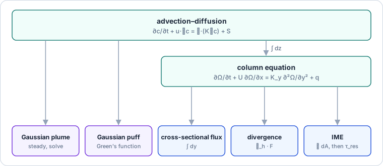
Figure 1:The five methods and the equation each comes from.
The Gaussian plume (plumax)
TL;DR. Solve (2) at steady state, integrate it over height, and invert the column for .
Problem. At steady state, plays the role of time (the travel time ), and (2) is a two-dimensional heat equation in , . Integrating (2) across turns the source into its initial condition, , so the source injects per metre of travel. With a reflecting ground and a release height ,
where and are the crosswind and vertical dispersion widths. The column of (4) is
which we invert for the emission rate on the plume’s axis:
1 2 3 4 5 6 7 8 9 10 11# Shapes: Q = 2 kg/s, U = 3 m/s, class D; x = 500, 1500 m # σ = a x (1 + b x)^c, Briggs, for y and z D = get_dispersion_params("D") # today # c(x, y, z) by (er1-eq-plume3d), with the image source c = plume_concentration(x, y, z, 0, 0, H, U, 0, Q, D) # today # Ω = ∫₀^∞ c dz, quadrature, H = 0 and 30 m (·) → () # → Q / (√(2π) U σ_y) e^{−y²/2σ_y²} to 10⁻⁶ user # σ_y: 39.0 m at 500 m, 146.1 m at 2 km # d ln σ_y / d ln x = 0.99 between 100 and 400 m # U ∬ c dy dz on a 1 m grid, H = 30 m (Y, Z) → () # → Q to 10⁻³ at 500 m and 1.5 km user
plumax’s 3D plume, integrated over height, against the column formula, from a real run.
The column formula (5) holds for any release height. The two image terms together integrate to whatever is, so plumax’s plume released at 30 m has the same column as one released at the ground, to quadrature accuracy. In addition, the flux through every cross-section, , is , which is simply the initial condition carried downwind (and the cross-sectional flux in three dimensions).
The Gaussian puff (plumax)
TL;DR. Release mass in puffs, keep along-wind diffusion, and recover the plume by superposition.
Problem. An instantaneous release of mass at and is the initial condition of (1), with afterwards. In the frame moving with the wind, , the chain rule cancels the advection term and leaves the heat equation . Its Green’s function is the product of three one-dimensional heat kernels, (with the -th coordinate of the moving frame), and with and an image at for a reflecting ground, we get
which is plumax’s puff_concentration, and its column is
again for any release height. A steady release is then the superposition of unit puffs, where each is (8) with .
1 2 3 4 5 6 7 8 9 10 11 12# Shapes: release ages a ∈ (0, 3600 s], 20,000 of them # Ω(x, 0) = ∫₀^T Q Ω₁(x, 0; a) da (a,) → () # against Q / (√(2π) U σ_y), σ_y² = 2 K x / U superposed(500, u=5) / kplume(500, u=5) # Pe 250 → 0.999 user superposed(50, u=5) / kplume(50, u=5) # Pe 25 → 0.990 user superposed(500, u=1) / kplume(500, u=1) # Pe 50 → 0.995 user superposed(50, u=1) / kplume(50, u=1) # Pe 5 → 0.958 user # plumax's puff, σ² = 2 K t, t = 100 s, H = 30 m, 2 m grid c = puff_concentration(x - U*t, y, z, 0, 0, H, σ, σ, σ, M) # today # ∭_{z ≥ 0} c dV = M to 10⁻⁶ (301, 301, 201) → () # ∫ c dz = (er1-eq-puffcol) to 10⁻⁶ (301, 301, 201) → (301, 301) # ∂c/∂t + U ∂c/∂x − K ∇²c = 0 to 10⁻⁴, central differences user
Puffs superposed against the steady plume, K = 10 m²/s, from a real run.
The puff sum and the plume agree to 0.1 % at a Péclet number of 250, and they differ by 4 % at 5, where the along-wind diffusion (which the plume drops) matters. So this is the note’s point about low winds made quantitative: the plume formula is the high-Péclet limit of the puff sum, not its exact steady state.
The cross-sectional flux (geotoolz)
TL;DR. Integrate the column across the plume at several downwind distances and multiply by the wind.
Problem. We integrate (3) at steady state over all . The diffusion term integrates to , because the plume and its gradient vanish far to the sides, and the source term integrates to :
which, with nothing upwind, integrates to
where is the step function. So the flux is constant downwind and equals :
When the wind varies with height, the flux through a transect is , so the wind that multiplies the column is the concentration-weighted one,
1 2 3 4 5 6 7 8 9 10# Shapes: 100 × 160 pixels at 20 m; transects every 400 m csf = gz.plume.CrossSectionalFlux( source=(0, 0), wind_u=3.0, wind_v=0.0, n_transects=5, transect_spacing_m=400) # today # Q_k = U Σ_j Ω_kj Δy (100, 160) → (5,) csf(column, x > 0)["flux_kg_s"] # → 2.000 ×5 today csf(column, column > 0.002)["flux_kg_s"] # thresholded today # → 1.90, 1.62, 1.25, 0.77, 0 # u(z) = 3 (z / 10 m)^0.15; U_eff = ∫ u c dz / ∫ c dz user # → 2.55 m/s at 100 m, 3.38 at 1 km, 3.62 at 2 km
geotoolz’s cross-sectional flux on the synthetic column, from a real run.
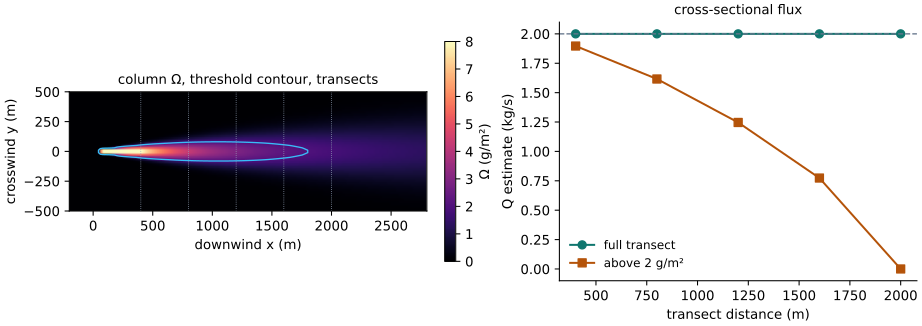
Figure 2:The cross-sectional flux on full and on thresholded transects.
On full transects the flux is at every distance, as (11) says (Figure 2). However, a detection threshold removes the plume’s flanks, and the far transects lose more: 5 % at 400 m, 61 % at 1.6 km, and everything at 2 km, where the whole transect is below 2 g/m². Shear changes the wind that applies, so a plume hugging the ground moves slower than the 10 m wind (2.55 against 3 m/s at 100 m) whereas a deeper one moves faster (3.62 at 2 km).
The divergence method (xrtoolz budgets)
TL;DR. Map the source as the divergence of the column flux, and check Gauss’s theorem on a box.
Problem. We write the column equation in flux form with the column flux , where are the horizontal wind and flux, and integrate it over a region which holds the source. Gauss’s theorem turns both divergences into boundary integrals, with the outward unit normal and the arc length along :
Averaged over a long period, and dropping the diffusive term, the source density is
and the emission rate of the region is
1 2 3 4 5 6 7 8 9 10# Shapes: F_x = U Ω (100, 160); boxes x ∈ [−100, 1500] m # q = ∂F_x/∂x, central differences (100, 160) → (100, 160) div = np.gradient(U * column, 20.0, axis=1) # user # Q_A = ∬_A q dA = ∮ F·n dl (100, 160) → () area_sum(box(-100, 1500, half=600)) # → 2.000 kg/s user area_sum(box(-100, 1500, half=60)) # → 0.81, too narrow # the dropped term on that box, K_eff = (U/2) dσ_y²/dx (Briggs) # 2 ∫₀^{x₁} K_eff Ω(x, h) h / σ_y² dx → 1.18; + 0.82 = Q user # one overpass, σ_Ω = 0.003 kg/m²: sd = U σ_Ω Δx √n_rows # → 1.39 kg/s (2,000 draws: 1.39; this draw 1.51); 49 for a 10 % sd
The divergence of the column flux on the grid, from a real run.
The area sum and the boundary flux agree to 10-6, as Gauss’s theorem requires, and a box wide enough to hold the plume returns . However, a box narrower than the plume returns 0.81 kg/s. The rest is the diffusive term of (13), which the method drops: plumax’s Briggs column solves the column equation with an effective diffusivity , and with it the diffusive flux through the narrow box’s side edges is 1.18 kg/s. The advective part (0.82 exactly, 0.81 on the grid) plus the diffusive part is to 10-6. So dropping diffusion is only safe for a boundary which crosses the plume where advection carries it (at the downwind edge) and lies outside it everywhere else. With noise, the area sum of a central difference telescopes to four edge columns, each weighted ½, so its uncertainty is theirs: 1.39 kg/s for one overpass at 0.003 kg/m² of noise (70 % of the signal), and 49 overpasses for a 10 % uncertainty. This is why the method averages many overpasses, as the note says it does at TROPOMI’s scale. xrtoolz’s budgets (control_volume_integral, boundary_flux) computes both sides of (15) on a model grid, but nothing in the stack applies them to methane columns yet.
The integrated mass enhancement (geotoolz)
TL;DR. Sum the mass above a detection threshold, divide by a residence time, and see what the boundary terms really are.
Problem. Let be the region where , for a detection threshold . On its boundary , so the advective boundary integral is
because the outward normal of a closed curve integrates to zero. Away from the source, the total flux balance of then leaves only diffusion, which means everything the source puts in leaves across the contour by crosswind diffusion,
The IME sidesteps the boundary with a residence time, , which is parameterised as . A scaling argument gives the same form from either balance. Balancing the source against advection, with , gives . Balancing it against what really leaves (the crosswind diffusion out of a plume of width and length ) gives , and the diffusive growth turns that into the same . The order-one factor which the scaling leaves out is what the calibration fixes. So, with and the column and the area of pixel ,
and the emission rate is
1 2 3 4 5 6 7 8 9 10 11 12# Shapes: K plume, K_y = 10 m²/s; contour Ω = 4 g/m², 663 m # ∮ U Ω n_x dl = −2 U Ω_thr [f(x_end) − f(0)] → 0 user # −∮ K_y ∂Ω/∂y n_y dl = 2 K_y Ω_thr ∫ f/σ² dx → 2.000 = Q user # IME = Σ Ω_j A_j over Ω > 2 g/m², plumax: 796 kg; τ_res = 398 s # L, chord of the mask (100, 160) → () L = plume_length(mask, transform, method="max_axis") # today # → 1,740 m; √A = 465 m # U_eff = Q L / IME: 1.17 m/s (√A), 4.37 m/s (chord) user # Q = U L⁻¹ IME, raw wind and chord (100, 160) → () ime = gz.plume.IMEEstimate(wind_speed=3.0, length_method="max_axis") # today ime(column, mask) # → 1.37 kg/s
The contour fluxes, and the IME with each plume length, from a real run.
Both contour integrals, (16) and (17), are exact: the advective flux through the contour is zero, and the diffusive flux is to 10-9. So the residence-time argument is not a way around small boundary terms. Instead, it replaces the one boundary term that carries the whole source (diffusion across the plume’s edge) with a calibrated wind, which is also why depends on the threshold, the noise and the turbulence, as the note says. The calibration is tied to the length scale it was fitted with: the same noise-free plume needs m/s with and 4.37 m/s with the chord, a factor of 3.7. geotoolz’s IMEEstimate, which computes (18) and (19), offers three length methods (max_axis by default, convex_hull and skeleton), and none of them is .
The five methods side by side
Table 1:The five methods, what each integrates and what each needs, with where it lives in the stack.
| Method | Integral of the equation | Assumes | Needs | Scale | In the stack today |
|---|---|---|---|---|---|
| Gaussian plume | none: solve (2) | steady state, constant , high Pe | wind speed and direction, stability | point source | plumax gauss_plume (Briggs, NumPyro inference) |
| Gaussian puff | superposition over release times | constant per puff | wind time series, | point source | plumax gauss_puff (Pasquill–Gifford or Briggs, time-varying wind) |
| Cross-sectional flux | on transects | steady state, full transects | wind speed and direction, shear | 50 m to 1 km | geotoolz plume.CrossSectionalFlux |
| Divergence | or | time average, no diffusion | gridded wind, many overpasses | 10 to 100 km | xrtoolz budgets (generic) |
| IME | , then | steady state, calibrated | wind speed, plume mask, the calibration’s | 50 m to 1 km | geotoolz plume.IMEEstimate |
The divergence method and the cross-sectional flux (Table 1) are the same statement in differential and in integral form. The IME is the area analogue of the cross-sectional flux, which trades the wind direction for a calibration. plumax also carries forward models that the note does not cover (a Lagrangian particle model and an Eulerian large-eddy model on finitevolx), which can generate the synthetic plumes an IME calibration is fitted on. The cross-sectional flux, the divergence method and the IME only use the column equation and not the Gaussian solution, so they hold for any plume shape.
Open questions
Which length does the stack’s IME calibration use? geotoolz takes as an input. The calibration and the length method should travel together as one object, so that a coefficient cannot meet a chord length.
Where should the divergence method live? It is a budget over a methane column on a grid, so xrtoolz’s budgets compute it, plumax owns the physics, and a TROPOMI pipeline owns the averaging.
Can plumax calibrate itself? Its large-eddy model can generate the synthetic plumes which Varon et al. made with WRF, and a calibration workflow would make the coefficients reproducible per instrument.
Upcoming work
Table 2 lists the follow-ups.
Table 2:Follow-ups from checking the source note.
| Follow-up | Where | Why |
|---|---|---|
Add length_method="sqrt_area" | geotoolz plume_length (plumax after the move) | the note’s and Varon et al.'s length is , which the operator cannot compute |
| Bundle with its length method | IMEEstimate | stage 5: a factor of 3.7 between two lengths on one plume |
| Report under shear in the cross-sectional flux | CrossSectionalFlux | stage 2: the effective wind is 15 % below the 10 m wind at 100 m and 21 % above it at 2 km |
| Add a methane divergence-method recipe on xrtoolz budgets | xrtoolz or plumax | nothing in the stack applies the method to columns |
References
The source note, “Emission Rate Estimation from First Principles” Johnson, 2026.
The IME and its calibration Varon et al., 2018, Sentinel-2 retrievals Varon et al., 2021, the airborne flux distribution Frankenberg & others, 2016, the cross-sectional flux Krings & others, 2011, the divergence method Beirle & others, 2019Liu & others, 2021Koene & others, 2024, the review Jacob & others, 2022 and the plume and puff comparison Jia et al., 2025.
plumax, geotoolz, georeader and xrtoolz at the revisions in the header.
- Johnson, J. E. (2026). Emission Rate Estimation from First Principles: the plume, the puff, the cross-sectional flux, the divergence method and the IME. Unpublished design note.
- Varon, D. J., Jacob, D. J., McKeever, J., Jervis, D., Durak, B. O. A., Xia, Y., & Huang, Y. (2018). Quantifying methane point sources from fine-scale satellite observations of atmospheric methane plumes. Atmospheric Measurement Techniques, 11(10), 5673–5686. 10.5194/amt-11-5673-2018
- Varon, D. J., Jervis, D., McKeever, J., Spence, I., Gains, D., & Jacob, D. J. (2021). High-frequency monitoring of anomalous methane point sources with multispectral Sentinel-2 satellite observations. Atmospheric Measurement Techniques, 14(4), 2771–2785. 10.5194/amt-14-2771-2021
- Frankenberg, C., & others. (2016). Airborne methane remote measurements reveal heavy-tail flux distribution in Four Corners region. Proceedings of the National Academy of Sciences, 113(35), 9734–9739. 10.1073/pnas.1605617113
- Krings, T., & others. (2011). MAMAP – a new spectrometer system for column-averaged methane and carbon dioxide observations from aircraft. Atmospheric Measurement Techniques, 4, 215–243. 10.5194/amt-4-215-2011
- Beirle, S., & others. (2019). Pinpointing nitrogen oxide emissions from space. Science Advances, 5, eaax9800. 10.1126/sciadv.aax9800
- Liu, M., & others. (2021). A new divergence method to quantify methane emissions using observations of Sentinel-5P TROPOMI. Geophysical Research Letters, 48, e2021GL094151. 10.1029/2021GL094151
- Koene, E., & others. (2024). On the theory of the divergence method for quantifying source emissions from satellite observations. Journal of Geophysical Research: Atmospheres, 129, e2023JD039904. 10.1029/2023JD039904
- Jacob, D. J., & others. (2022). Quantifying methane emissions from the global scale down to point sources using satellite observations of atmospheric methane. Atmospheric Chemistry and Physics, 22, 9617–9646. 10.5194/acp-22-9617-2022
- Jia, M., Daniels, W., & Sprinkle, B. (2025). Comparison of the Gaussian plume and puff atmospheric dispersion models for methane modeling on oil and gas sites. Scientific Reports, 15.