1D Example Walk-through

Colab Notebooks

Name	Colab Notebook
scikit-learn
GPFlow
GPyTorch

This post we will go over a 1D example where I show how one can fit a Gaussian process using the scikit-learn, GPFlow and GPyTorch libraries. Each of these libraries range in complexity with scikit-learn being the simplest, GPyTorch being the most complicated and GPFlow being somewhere in between. For newcomers, it's good to see the differences before making your decision.

In this demo, we will do a small data problem; just 25 samples. This is where a GP tends to excel because of

---

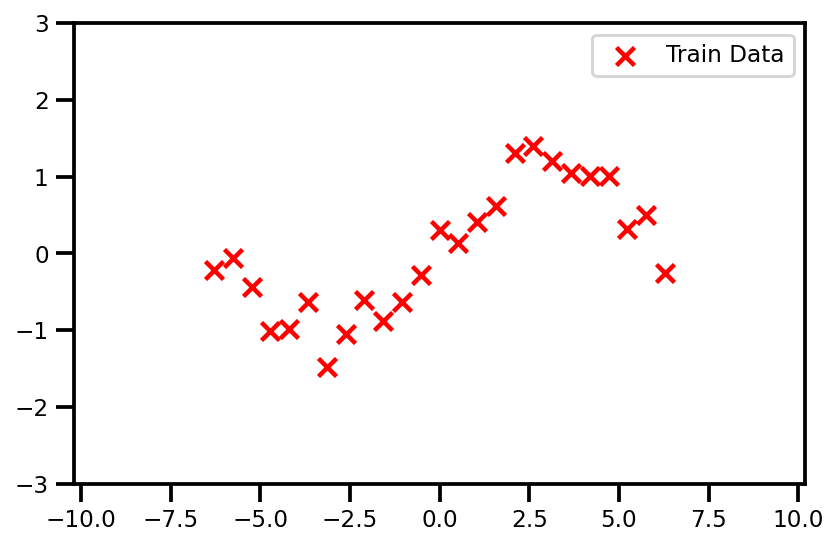
Data

The way we generate the data will be the same for all packages. Here is the code and demo data that we're working with;

Code

# control the seed
seed = 123
rng = np.random.RandomState(seed)

# Generate sample data
n_samples = 25

def f(x):
    return np.sin(0.5 * X)

X = np.linspace(-2*np.pi, 2*np.pi, n_samples)
y =  f(X) + 0.2 * rng.randn(X.shape[0])

X, y = X[:, np.newaxis], y[:, np.newaxis]

plt.figure()
plt.scatter(X, y, label="Train Data")
plt.legend()
plt.show()

---

GP Model

Scikit-Learn

In scikit-learn we just need the .fit(), .predict(), and .score().

First we need to define the parameters necessary for the gaussian process regression algorithm

from sklearn.gaussian_process import GaussianProcessRegressor
from sklearn.gaussian_process.kernels import RBF, WhiteKernel, ConstantKernel

# define the kernel
kernel = ConstantKernel() * RBF() + WhiteKernel()

# define the model
gp_model = GaussianProcessRegressor(
    kernel=kernel,          # Kernel Function
    alpha=1e-5,             # Noise Level
    n_restarts_optimizer=5  # Good Practice
)

GPFlow

Mean & Kernel Function

So GPflow gives us some extra flexibility. We need to have a all the moving parts to define our standard GP.

from gpflow.mean_functions import Linear
from gpflow.kernels import RBF

# define mean function
mean_f = Linear()

# define the kernel
kernel = RBF()

GP Model

from gpflow.models import GPR

# define GP Model
gp_model = GPR(data=(X, y), kernel=kernel, mean_function=mean_f)

# get a nice summary
print_summary(gp_model, )

╒═════════════════════════╤═══════════╤══════════════════╤═════════╤═════════════╤═════════╤═════════╤═════════╕
│ name                    │ class     │ transform        │ prior   │ trainable   │ shape   │ dtype   │ value   │
╞═════════════════════════╪═══════════╪══════════════════╪═════════╪═════════════╪═════════╪═════════╪═════════╡
│ GPR.mean_function.A     │ Parameter │ Identity         │         │ True        │ (1, 1)  │ float64 │ [[1.]]  │
├─────────────────────────┼───────────┼──────────────────┼─────────┼─────────────┼─────────┼─────────┼─────────┤
│ GPR.mean_function.b     │ Parameter │ Identity         │         │ True        │ (1,)    │ float64 │ [0.]    │
├─────────────────────────┼───────────┼──────────────────┼─────────┼─────────────┼─────────┼─────────┼─────────┤
│ GPR.kernel.variance     │ Parameter │ Softplus         │         │ True        │ ()      │ float64 │ 1.0     │
├─────────────────────────┼───────────┼──────────────────┼─────────┼─────────────┼─────────┼─────────┼─────────┤
│ GPR.kernel.lengthscales │ Parameter │ Softplus         │         │ True        │ ()      │ float64 │ 1.0     │
├─────────────────────────┼───────────┼──────────────────┼─────────┼─────────────┼─────────┼─────────┼─────────┤
│ GPR.likelihood.variance │ Parameter │ Softplus + Shift │         │ True        │ ()      │ float64 │ 1.0     │

Numpy 2 Tensor

Notice how I didn't do anything about changing from the np.ndarray to the tf.tensor? Well that's because GPFlow is awesome and does it for you. Little things like that make the coding experience so much better.

GPyTorch

Numpy to Tensor

Unfortunately, this is one of those things where PyTorch becomes more involved to use. There is no automatic conversion from a np.ndarray to a torch.Tensor. So in your code bases, you need to ensure that you do this.

# convert to tensor
X_tensor, y_tensor = torch.Tensor(X.squeeze()), torch.Tensor(y.squeeze())

Define GP Model

Again, this is involved. You need to create the GP model exactly how one would think about doing it. You need a mean function, a kernel function, a likelihood and some data. We inherit the gpytorch.models.ExactGP class and we're good to go.

# We will use the simplest form of GP model, exact inference
class GPModel(gpytorch.models.ExactGP):
    def __init__(self, train_x, train_y, likelihood, mean_module, covar_module):
        super().__init__(train_x, train_y, likelihood)
        # Constant Mean function
        self.mean_module = mean_module
        # RBF Kernel Function
        self.covar_module = covar_module

    def forward(self, x):
        mean_x = self.mean_module(x)
        covar_x = self.covar_module(x)
        return gpytorch.distributions.MultivariateNormal(mean_x, covar_x)

Initialize GP model

Now that we've defined our GP, we can intialize it with the appropriate parameters - mean function, kernel function and likelihood.

# initialize mean function
mean_f = gpytorch.means.ConstantMean()

# initialize kernel function
kernel = gpytorch.kernels.ScaleKernel(gpytorch.kernels.RBFKernel())

# intialize the likelihood
likelihood = gpytorch.likelihoods.GaussianLikelihood()

# initialize the gp model with the likelihood
gp_model = GPModel(X_tensor, y_tensor, likelihood, mean_f, kernel)

And we're done! So now you noticed that you learned a bit more than necessary to actually understand how the GP works because you had to build it from scratch (to some extent). This can be cumbersome but it might be more useful than the sklearn implementation because it gives us a bit more flexibility.

---

Training Step

Training Time

Data Points	scikit-learn	GPFlow	GPyTorch
25	0.009 secs	0.352 secs	0.328 secs
100	0.044 secs	0.339 secs	0.735 secs
500	0.876 secs	1.47 secs	3.14 secs
1,000	3.93 secs	6.5 secs	4.5 secs
2,000	17.7 secs	32 secs	16 secs

Scikit-Learn

It doesn't get any simpler than this...

# fit GP model
gp_model.fit(X, y);

It's because everything is under the hood within the .fit method.

GPFlow

# define optimizer and params
opt = gpflow.optimizers.Scipy()
method = "L-BFGS-B"
n_iters = 100

# optimize
opt_logs = opt.minimize(
    gp_model.training_loss,
    gp_model.trainable_variables, 
    options=dict(maxiter=n_iters),
    method=method,
)

# print a summary of the results
print_summary(gp_model)

╒═════════════════════════╤═══════════╤══════════════════╤═════════╤═════════════╤═════════╤═════════╤═════════════════════╕
│ name                    │ class     │ transform        │ prior   │ trainable   │ shape   │ dtype   │ value               │
╞═════════════════════════╪═══════════╪══════════════════╪═════════╪═════════════╪═════════╪═════════╪═════════════════════╡
│ GPR.mean_function.A     │ Parameter │ Identity         │         │ True        │ (1, 1)  │ float64 │ [[-0.053]]          │
├─────────────────────────┼───────────┼──────────────────┼─────────┼─────────────┼─────────┼─────────┼─────────────────────┤
│ GPR.mean_function.b     │ Parameter │ Identity         │         │ True        │ (1,)    │ float64 │ [-0.09]             │
├─────────────────────────┼───────────┼──────────────────┼─────────┼─────────────┼─────────┼─────────┼─────────────────────┤
│ GPR.kernel.variance     │ Parameter │ Softplus         │         │ True        │ ()      │ float64 │ 1.0576019909271173  │
├─────────────────────────┼───────────┼──────────────────┼─────────┼─────────────┼─────────┼─────────┼─────────────────────┤
│ GPR.kernel.lengthscales │ Parameter │ Softplus         │         │ True        │ ()      │ float64 │ 3.3182129463115735  │
├─────────────────────────┼───────────┼──────────────────┼─────────┼─────────────┼─────────┼─────────┼─────────────────────┤
│ GPR.likelihood.variance │ Parameter │ Softplus + Shift │         │ True        │ ()      │ float64 │ 0.05877109253391096 │
╘═════════════════════════╧═══════════╧══════════════════╧═════════╧═════════════╧═════════╧═════════╧═════════════════════╛

GPyTorch

So admittedly, this is where we start to enter into boilerplate code because this is stuff that needs to be done almost always.

Set Model and Likelihood in Training Mode

For this step, we need to let PyTorch know that we want all of the layers inside of our class primed and ready in train mode.

Note

This is mostly from things like BatchNormalization and DropOut which tend to behave differently between train and test. But we inherited the commands.

# set model and likelihood in train mode
likelihood.train()
gp_model.train()

One nice thing is that it will give you a small overview of how the model looks as a tuple of tuples.

GPModel(
(likelihood): GaussianLikelihood(
    (noise_covar): HomoskedasticNoise(
    (raw_noise_constraint): GreaterThan(1.000E-04)
    )
)
(mean_module): ConstantMean()
(covar_module): ScaleKernel(
    (base_kernel): RBFKernel(
    (raw_lengthscale_constraint): Positive()
    )
    (raw_outputscale_constraint): Positive()
)
)

Choose Optimizer and Loss

Now we define the optimizer as well as the loss function.

# optimizer setup
lr = 0.1

# Use the adam optimizer
optimizer = torch.optim.Adam(
    gp_model.parameters(), lr=lr
) 

# Loss Function - the marginal log likelihood
mll = gpytorch.mlls.ExactMarginalLogLikelihood(likelihood, gp_model)

Training

And now we can finally train our model! Now, all of this that comes after is boilerplate code. We have to do it almost every time when using PyTorch. No escaping unless you want to use another package (which you should; I'll demonstrate that in a later tutorial).

# choose iterations
n_epochs = 100

# initialize progressbar
with tqdm.notebook.trange(n_epochs) as pbar:
    for i in pbar:
        # Zero gradients from previous iteration
        optimizer.zero_grad()

        # Output from model
        output = gp_model(X_tensor)
        # Calc loss
        loss = -mll(output, y_tensor)

        # backprop gradients
        loss.backward()

        # get parameters we want to track
        postfix = dict(
            Loss=loss.item(),
            scale=gp_model.covar_module.outputscale.item(),
            length_scale=gp_model.covar_module.base_kernel.lengthscale.item(),
            noise=gp_model.likelihood.noise.item()
            )

        # step forward in the optimization
        optimizer.step()

        # update the progress bar
        pbar.set_postfix(postfix)

---

Predictions

Scikit-Learn

Predictions are also very simple. You simply call the .predict method and you will get your predictive mean. If you want the predictive variance, you need to put the return_std flag as True.

# generate some points for plotting
X_plot = np.linspace(- 1.2, 1.2, 100)[:, np.newaxis]

# predictive mean and standard deviation
y_mean, y_std = gp_model.predict(X_plot, return_std=True)

# confidence intervals
y_upper = y_mean.squeeze() + 2* y_std
y_lower = y_mean.squeeze() - 2* y_std

Predictive Standard Deviation

There is no way to turn off or no the likelihood noise or not (i.e. the predictive mean y of the predictive mean f). It is always y so the standard deviations will be a little high. To not use the y, you will need to actually subtract the WhiteKernel and the alpha from your predictive standard deviation.

GPFlow

# generate some points for plotting
X_plot = np.linspace(-3*np.pi, 3*np.pi, 100)[:, np.newaxis]

# predictive mean and standard deviation
y_mean, y_var = gp_model.predict_y(X_plot)

# convert to numpy arrays
y_mean, y_var = y_mean.numpy(), y_var.numpy()

# confidence intervals
y_upper = y_mean + 2* np.sqrt(y_var)
y_lower = y_mean - 2* np.sqrt(y_var)

Tensor 2 Numpy

So we do have to convert to numpy arrays from tensors for the predictions. Note, you can plot tensors, but some of the commands might be different.

E.g.

y_upper = tf.squeeze(y_mean + 2 * tf.sqrt(y_var))

GPyTorch

We're still now out of it yet. We still need to do a few extra stuff to get predictions. Here we can simply

Eval Mode

We need to put our model back in .eval mode. This will allow all layers to behave in eval mode.

# put the model in eval mode
gp_model.eval()
likelihood.eval()

One nice thing is that the resulting observed_pred is actually a class with a few methods and properties, e.g. mean, variance, confidence_region. Very convenient for predictions.

# generate some points for plotting
X_plot = np.linspace(-3*np.pi, 3*np.pi, 100)[:, np.newaxis]

# convert to tensor
X_plot_tensor = torch.Tensor(X_plot)


# turn off the gradient-tracking
with torch.no_grad():

    # generate data
    X_plot_tensor = torch.linspace(-3*np.pi, 3*np.pi, 100)

    # get predictions
    observed_pred = likelihood(gp_model(X_plot_tensor))

    # extract mean prediction
    y_mean_tensor = observed_pred.mean

    # extract confidence intervals
    y_upper_tensor, y_lower_tensor = observed_pred.confidence_region()

And yes...we still have to convert our data to np.ndarray.

# convert to numpy array
X_plot = X_plot_tensor.numpy()
y_mean = y_mean_tensor.numpy()
y_upper = y_upper_tensor.numpy()
y_lower = y_lower_tensor.numpy()

---

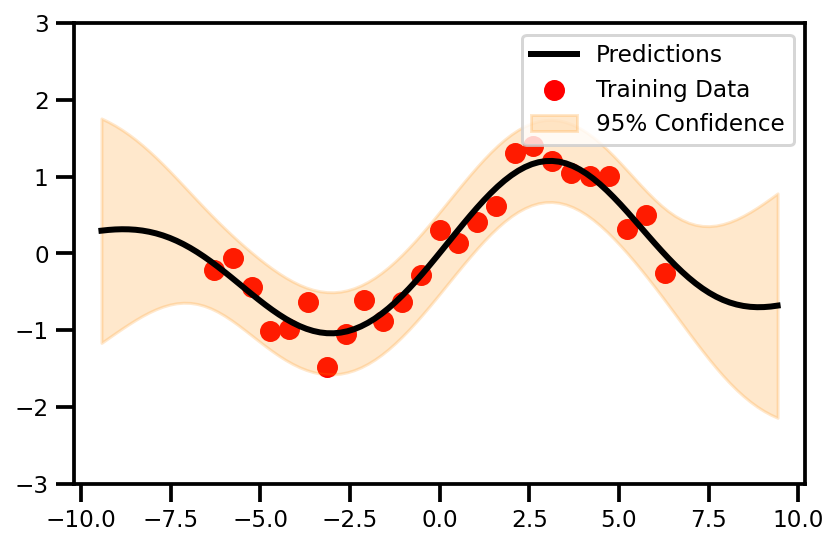
Visualization

Plot Function

It's the same for all libraries as I first convert everything to numpy arrays and then plot the results.

fig, ax = plt.subplots()

ax.scatter(
    X, y, 
    label="Training Data",
    color='Red'
)

ax.plot(
    X_plot, y_mean, 
    color='black', lw=3, label='Predictions'
)
plt.fill_between(
    X_plot.squeeze(), 
    y_upper.squeeze(), 
    y_lower.squeeze(), 
    color='darkorange', alpha=0.2,
    label='95% Confidence'
)
ax.set_ylim([-3, 3])
ax.set_xlim([-10.2, 10.2])
ax.legend()
plt.tight_layout()
plt.show()

Scikit-Learn

GPFlow

GPyTorch