Large Scale 1D Example Walk-through

Colab Notebooks

Name	Colab Notebook
scikit-learn
GPFlow
GPyTorch

This demo we will demonstrate how different algorithms compare when

---

Background

In exact GP estimation, we try to minimize the negative marginal log-likelihood term given by:

$$\log \mathcal{N}(y | 0, K + \sigma^2I) = - \frac{1}{2} y^\top\left( K + \sigma^2I \right)^{-1}y - \frac{1}{2}\log \left| K + \sigma^2 \right| - \frac{n}{2}\log 2\pi$$

So typically any exact GP estimation, there will be two expensive parts to this algorithm: $K^{-1}$ and $\log |K|$ which has a computational cost of $\mathcal{O}(N^3)$. This is bad and very expensive. Unless you have Google Cloud Platform computational services, you will suffer on a graduate student's laptop. We're talking an upper limit of 10K points if you're willing to be patient.

Method 1 - Sparse

One thing we can do is to reduce the amount of points that we invert. These representative points are known as inducing points. This results in the Nyström approximation which changes our likelihood term from $\log p(y|X,\theta)$ to:

$$\log \mathcal{N}(y | 0, K + \sigma^2I) \approx \log \mathcal{N}(y | 0, \tilde{K} + \sigma^2I)$$

Notice how we haven't actually changing our formulation because we still have to calculate the inverse of $\tilde{K}$ which is $\mathbb{R}^{N \times N}$. Using the Woodbury matrix identity for the kernel approximation form (Sherman-Morrison Formula):

$$(\tilde{K} + \sigma^2 I)^{-1}=\sigma^{-2}I - \sigma^{-4}K_z(K_{zz}+\sigma^{-2}K_z^{\top}K_z)^{-1}K_z^{\top}$$

Now the matrix that we need to invert is $(K_{zz}+\sigma^{-2}K_z^{\top}K_z)^{-1}$ which is $(M \times M)$ which is considerably smaller if $M << N$. So the overall computational complexity reduces from $\mathcal{O}(N^3)$ to $\mathcal{O}(MN^2)$ where $M<<N$ $\mathcal{O}(NM^2)$.

Method 2 - Black-Box Matrix-Matrix (BBMM)

This uses good ol' matrix multiplication strategies that you saw in your numerical methods class but perhaps never paid attention to. It uses a modified batched version of the conjugate gradients for the most expensive parts of the algorithm. It also uses preconditioning strategies to speed up the convergence. So remember, GPU acceleration is powerful because it's comprised of many cores that utilize matrix multiplication. So this is why this is much faster and it scales in the settings of GPUs. So the overall computational complexity reduces from $\mathcal{O}(N^3)$ to $\mathcal{O}(N^2)$.

Below, let's see how these methods do in approximating a 1D dataset in terms of speed.

---

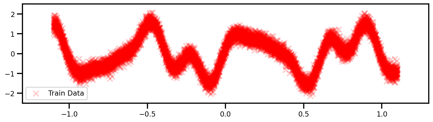
Data

Let's generate a more complex example which would definitely require more than 25 data points to capture. (OK, Maybe not 10K but enough)...

$$f(x) = \sin(3\pi x) + \frac{1}{3}\sin(9\pi x) + \frac{1}{2} \sin(7 \pi x)$$

Code

n_samples = 10_000

def f(x):
    return np.sin(x * 3 * 3.14) + 0.3 * np.cos(x * 9 * 3.14) + 0.5 * np.sin(x * 7 * 3.14)

X = np.linspace(-1.1, 1.1, n_samples)
X_plot = np.linspace(- 1.3, 1.3, 100)[:, np.newaxis]
y =  f(X) + 0.2 * rng.randn(X.shape[0])

X, y = X[:, np.newaxis], y[:, np.newaxis]

10,000 Data Points!

Source: GPFlow - Big Data Tutorial

---

GP Model

For this example, we'll just show the 3 different methods using the standard linear mention function and the RBF kernel matrix.. The code will be very identical. The only major difference is that the sparse approximations need some inducing points (representative points).

GPFlow (Exact)

from gpflow.mean_functions import Linear
from gpflow.kernels import RBF
from gpflow.models import GPR

# define the kernel
kernel = RBF()

# define mean function
mean_f = Linear()

# define GP Model
gp_model = GPR(data=(X, y), kernel=kernel, mean_function=mean_f)

GPFlow (Sparse)

Kernel & Mean Function

from gpflow.mean_functions import Linear
from gpflow.kernels import RBF

# define the kernel
kernel = RBF()

# define mean function
mean_f = Linear()

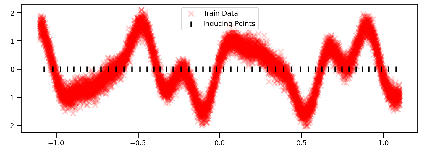
Inducing Points

from sklearn.cluster import KMeans

n_inducing = 50
seed = 123

# KMeans model
kmeans_clf = KMeans(n_clusters=n_inducing)
kmeans_clf.fit(X)

# get cluster centers as inducing points
Z = kmeans_clf.cluster_centers_

GP Model

from gpflow.models import SGPR

# define GP Model
sgpr_model = SGPR(
    data=(X, y),
    kernel=kernel,
    inducing_variable=Z,
    mean_function=mean_f, 
)


# get a nice summary
print_summary(sgpr_model, )

╒══════════════════════════╤═══════════╤══════════════════╤═════════╤═════════════╤═════════╤═════════╤════════════╕
│ name                     │ class     │ transform        │ prior   │ trainable   │ shape   │ dtype   │ value      │
╞══════════════════════════╪═══════════╪══════════════════╪═════════╪═════════════╪═════════╪═════════╪════════════╡
│ SGPR.mean_function.A     │ Parameter │ Identity         │         │ True        │ (1, 1)  │ float64 │ [[1.]]     │
├──────────────────────────┼───────────┼──────────────────┼─────────┼─────────────┼─────────┼─────────┼────────────┤
│ SGPR.mean_function.b     │ Parameter │ Identity         │         │ True        │ (1,)    │ float64 │ [0.]       │
├──────────────────────────┼───────────┼──────────────────┼─────────┼─────────────┼─────────┼─────────┼────────────┤
│ SGPR.kernel.variance     │ Parameter │ Softplus         │         │ True        │ ()      │ float64 │ 1.0        │
├──────────────────────────┼───────────┼──────────────────┼─────────┼─────────────┼─────────┼─────────┼────────────┤
│ SGPR.kernel.lengthscales │ Parameter │ Softplus         │         │ True        │ ()      │ float64 │ 1.0        │
├──────────────────────────┼───────────┼──────────────────┼─────────┼─────────────┼─────────┼─────────┼────────────┤
│ SGPR.likelihood.variance │ Parameter │ Softplus + Shift │         │ True        │ ()      │ float64 │ 1.0        │
├──────────────────────────┼───────────┼──────────────────┼─────────┼─────────────┼─────────┼─────────┼────────────┤
│ SGPR.inducing_variable.Z │ Parameter │ Identity         │         │ True        │ (50, 1) │ float64 │ [[0.118... │
╘══════════════════════════╧═══════════╧══════════════════╧═════════╧═════════════╧═════════╧═════════╧════════════╛

Numpy 2 Tensor

Notice how I didn't do anything about changing from the np.ndarray to the tf.tensor? Well that's because GPFlow is awesome and does it for you. Little things like that make the coding experience so much better.

GPyTorch (Exact BBMM)

Numpy to Tensor

Unfortunately, this is one of those things where PyTorch becomes more involved to use. There is no automatic conversion from a np.ndarray to a torch.Tensor. So in your code bases, you need to ensure that you do this.

# convert to tensor
X_tensor, y_tensor = torch.Tensor(X.squeeze()), torch.Tensor(y.squeeze())

Define GP Model

Again, this is involved. You need to create the GP model exactly how one would think about doing it. You need a mean function, a kernel function, a likelihood and some data. We inherit the gpytorch.models.ExactGP class and we're good to go.

# We will use the simplest form of GP model, exact inference
class GPModel(gpytorch.models.ExactGP):
    def __init__(self, train_x, train_y, likelihood, mean_module, covar_module):
        super().__init__(train_x, train_y, likelihood)
        # Constant Mean function
        self.mean_module = mean_module
        # RBF Kernel Function
        self.covar_module = covar_module

    def forward(self, x):
        mean_x = self.mean_module(x)
        covar_x = self.covar_module(x)
        return gpytorch.distributions.MultivariateNormal(mean_x, covar_x)

Initialize GP model

Now that we've defined our GP, we can intialize it with the appropriate parameters - mean function, kernel function and likelihood.

# initialize mean function
mean_f = gpytorch.means.ConstantMean()

# initialize kernel function
kernel = gpytorch.kernels.ScaleKernel(gpytorch.kernels.RBFKernel())

# intialize the likelihood
likelihood = gpytorch.likelihoods.GaussianLikelihood()

# initialize the gp model with the likelihood
gp_model = GPModel(X_tensor, y_tensor, likelihood, mean_f, kernel)

And we're done! So now you noticed that you learned a bit more than necessary to actually understand how the GP works because you had to build it from scratch (to some extent). This can be cumbersome but it might be more useful than the sklearn implementation because it gives us a bit more flexibility.

GPU

So to get some scaling and faster training, we can use the GPU. For PyTorch, that means converting everything to a Tensor format.

X_tensor = X_tensor.cuda()
y_tensor = y_tensor.cuda()
gp_model = gp_model.cuda()
likelihood = likelihood.cuda()

---

Training Step

Training Time

GPFlow (Exact)	GPFlow (Sparse)	GPyTorch (Exact)
24 minutes	3 seconds	30 seconds
GPU	GPU	GPU

GPFlow (Exact)

# define optimizer and params
opt = gpflow.optimizers.Scipy()
method = "L-BFGS-B"
n_iters = 100

# optimize
opt_logs = opt.minimize(
    gp_model.training_loss,
    gp_model.trainable_variables, 
    options=dict(maxiter=n_iters),
    method=method,
)

# print a summary of the results
print_summary(gp_model)

╒═════════════════════════╤═══════════╤══════════════════╤═════════╤═════════════╤═════════╤═════════╤═════════════════════╕
│ name                    │ class     │ transform        │ prior   │ trainable   │ shape   │ dtype   │ value               │
╞═════════════════════════╪═══════════╪══════════════════╪═════════╪═════════════╪═════════╪═════════╪═════════════════════╡
│ GPR.mean_function.A     │ Parameter │ Identity         │         │ True        │ (1, 1)  │ float64 │ [[-0.109]]          │
├─────────────────────────┼───────────┼──────────────────┼─────────┼─────────────┼─────────┼─────────┼─────────────────────┤
│ GPR.mean_function.b     │ Parameter │ Identity         │         │ True        │ (1,)    │ float64 │ [-0.027]            │
├─────────────────────────┼───────────┼──────────────────┼─────────┼─────────────┼─────────┼─────────┼─────────────────────┤
│ GPR.kernel.variance     │ Parameter │ Softplus         │         │ True        │ ()      │ float64 │ 1.4583605690651238  │
├─────────────────────────┼───────────┼──────────────────┼─────────┼─────────────┼─────────┼─────────┼─────────────────────┤
│ GPR.kernel.lengthscales │ Parameter │ Softplus         │         │ True        │ ()      │ float64 │ 0.10119699753609418 │
├─────────────────────────┼───────────┼──────────────────┼─────────┼─────────────┼─────────┼─────────┼─────────────────────┤
│ GPR.likelihood.variance │ Parameter │ Softplus + Shift │         │ True        │ ()      │ float64 │ 0.03981121449717302 │
╘═════════════════════════╧═══════════╧══════════════════╧═════════╧═════════════╧═════════╧═════════╧═════════════════════╛
CPU times: user 13min 42s, sys: 9min 57s, total: 23min 40s
Wall time: 24min 43s

GPFlow (Sparse)

# define optimizer and params
minibatch_size = 128

# turn of training for inducing points
opt = gpflow.optimizers.Scipy()

# training loss
training_loss = sgpr_model.training_loss_closure()
method = "L-BFGS-B"
n_iters = 1_000

# optimize
opt_logs = opt.minimize(
    sgpr_model.training_loss,
    sgpr_model.trainable_variables, 
    options=dict(maxiter=n_iters),
    method=method,
)

# print a summary of the results
print_summary(sgpr_model)

╒══════════════════════════╤═══════════╤══════════════════╤═════════╤═════════════╤═════════╤═════════╤═════════════════════╕
│ name                     │ class     │ transform        │ prior   │ trainable   │ shape   │ dtype   │ value               │
╞══════════════════════════╪═══════════╪══════════════════╪═════════╪═════════════╪═════════╪═════════╪═════════════════════╡
│ SGPR.mean_function.A     │ Parameter │ Identity         │         │ True        │ (1, 1)  │ float64 │ [[-0.111]]          │
├──────────────────────────┼───────────┼──────────────────┼─────────┼─────────────┼─────────┼─────────┼─────────────────────┤
│ SGPR.mean_function.b     │ Parameter │ Identity         │         │ True        │ (1,)    │ float64 │ [-0.027]            │
├──────────────────────────┼───────────┼──────────────────┼─────────┼─────────────┼─────────┼─────────┼─────────────────────┤
│ SGPR.kernel.variance     │ Parameter │ Softplus         │         │ True        │ ()      │ float64 │ 1.4608235231409987  │
├──────────────────────────┼───────────┼──────────────────┼─────────┼─────────────┼─────────┼─────────┼─────────────────────┤
│ SGPR.kernel.lengthscales │ Parameter │ Softplus         │         │ True        │ ()      │ float64 │ 0.10123051205205866 │
├──────────────────────────┼───────────┼──────────────────┼─────────┼─────────────┼─────────┼─────────┼─────────────────────┤
│ SGPR.likelihood.variance │ Parameter │ Softplus + Shift │         │ True        │ ()      │ float64 │ 0.03980796876613383 │
├──────────────────────────┼───────────┼──────────────────┼─────────┼─────────────┼─────────┼─────────┼─────────────────────┤
│ SGPR.inducing_variable.Z │ Parameter │ Identity         │         │ True        │ (50, 1) │ float64 │ [[0.107...          │
╘══════════════════════════╧═══════════╧══════════════════╧═════════╧═════════════╧═════════╧═════════╧═════════════════════╛
CPU times: user 2.01 s, sys: 196 ms, total: 2.21 s
Wall time: 2.24 s══════════╧═════════╧═════════════╧═════════╧═════════╧═════════════════════╛

GPyTorch (Exact BBMM)

Same as small data

So this code is actually the same as the small data 1D Example! We just have to change it to use the GPU and we're good to go!

So admittedly, this is where we start to enter into boilerplate code because this is stuff that needs to be done almost always.

Set Model and Likelihood in Training Mode

For this step, we need to let PyTorch know that we want all of the layers inside of our class primed and ready in train mode.

Note

This is mostly from things like BatchNormalization and DropOut which tend to behave differently between train and test. But we inherited the commands.

# set model and likelihood in train mode
likelihood.train()
gp_model.train()

One nice thing is that it will give you a small overview of how the model looks as a tuple of tuples.

GPModel(
(likelihood): GaussianLikelihood(
    (noise_covar): HomoskedasticNoise(
    (raw_noise_constraint): GreaterThan(1.000E-04)
    )
)
(mean_module): ConstantMean()
(covar_module): ScaleKernel(
    (base_kernel): RBFKernel(
    (raw_lengthscale_constraint): Positive()
    )
    (raw_outputscale_constraint): Positive()
)
)

Choose Optimizer and Loss

Now we define the optimizer as well as the loss function.

# optimizer setup
lr = 0.1

# Use the adam optimizer
optimizer = torch.optim.Adam(
    gp_model.parameters(), lr=lr
) 

# Loss Function - the marginal log likelihood
mll = gpytorch.mlls.ExactMarginalLogLikelihood(likelihood, gp_model)

Training

And now we can finally train our model! Now, all of this that comes after is boilerplate code. We have to do it almost every time when using PyTorch. No escaping unless you want to use another package (which you should; I'll demonstrate that in a later tutorial).

# choose iterations
n_epochs = 100

# initialize progressbar
with tqdm.notebook.trange(n_epochs) as pbar:
    for i in pbar:
        # Zero gradients from previous iteration
        optimizer.zero_grad()

        # Output from model
        output = gp_model(X_tensor)
        # Calc loss
        loss = -mll(output, y_tensor)

        # backprop gradients
        loss.backward()

        # get parameters we want to track
        postfix = dict(
            Loss=loss.item(),
            scale=gp_model.covar_module.outputscale.item(),
            length_scale=gp_model.covar_module.base_kernel.lengthscale.item(),
            noise=gp_model.likelihood.noise.item()
            )

        # step forward in the optimization
        optimizer.step()

        # update the progress bar
        pbar.set_postfix(postfix)

---

Predictions

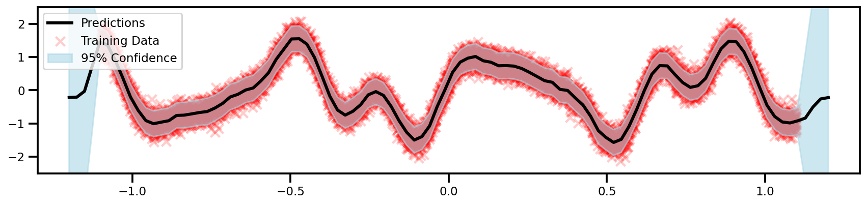
GPFlow (Exact)

# generate some points for plotting
X_plot = np.linspace(-3*np.pi, 3*np.pi, 100)[:, np.newaxis]

# predictive mean and standard deviation
y_mean, y_var = gp_model.predict_y(X_plot)

# convert to numpy arrays
y_mean, y_var = y_mean.numpy(), y_var.numpy()

# confidence intervals
y_upper = y_mean + 2* np.sqrt(y_var)
y_lower = y_mean - 2* np.sqrt(y_var)

Tensor 2 Numpy

So we do have to convert to numpy arrays from tensors for the predictions. Note, you can plot tensors, but some of the commands might be different.

E.g.

y_upper = tf.squeeze(y_mean + 2 * tf.sqrt(y_var))

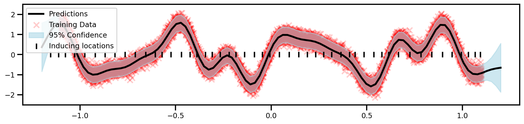
GPFlow (Sparse)

# generate some points for plotting
X_plot = np.linspace(-1.2, 1.2, 100)[:, np.newaxis]

# predictive mean and standard deviation
y_mean, y_var = sgpr_model.predict_y(X_plot)


# convert to numpy arrays
y_mean, y_var = y_mean.numpy(), y_var.numpy()

# confidence intervals
y_upper = y_mean + 2* np.sqrt(y_var)
y_lower = y_mean - 2* np.sqrt(y_var)

# Get learned inducing points
Z = sgpr_model.inducing_variable.Z.numpy()

Tensor 2 Numpy

So we do have to convert to numpy arrays from tensors for the predictions. Note, you can plot tensors, but some of the commands might be different.

E.g.

y_upper = tf.squeeze(y_mean + 2 * tf.sqrt(y_var))

GPyTorch (Exact BBMM)

Same as small data

Again, this code is actually the same as the small data 1D Example! We just have to port our input data to the GPU (always)!

We're still now out of it yet. We still need to do a few extra stuff to get predictions. Here we can simply

Eval Mode

We need to put our model back in .eval mode. This will allow all layers to behave in eval mode.

# put the model in eval mode
gp_model.eval()
likelihood.eval()

One nice thing is that the resulting observed_pred is actually a class with a few methods and properties, e.g. mean, variance, confidence_region. Very convenient for predictions.

# generate some points for plotting
X_plot = np.linspace(-3*np.pi, 3*np.pi, 100)[:, np.newaxis]

# convert to tensor
X_plot_tensor = torch.Tensor(X_plot)


# turn off the gradient-tracking
with torch.no_grad():

    # generate data
    X_plot_tensor = torch.linspace(-3*np.pi, 3*np.pi, 100)

    # convert tensor to CUDA
    X_plot_tensor = X_plot_tensor.cuda()

    # get predictions
    observed_pred = likelihood(gp_model(X_plot_tensor))

    # extract mean prediction
    y_mean_tensor = observed_pred.mean

    # extract confidence intervals
    y_upper_tensor, y_lower_tensor = observed_pred.confidence_region()

And yes...we still have to convert our data to np.ndarray.

# convert to numpy array
X_plot = X_plot_tensor.numpy()
y_mean = y_mean_tensor.numpy()
y_upper = y_upper_tensor.numpy()
y_lower = y_lower_tensor.numpy()

---

Visualization

Plot Function

It's the same for all libraries as I first convert everything to numpy arrays and then plot the results.

fig, ax = plt.subplots(figsize=(12, 4))

ax.scatter(
    X, y, 
    label="Training Data",
    color='Red',
    marker='x',
    alpha=0.2
)

ax.plot(
    X_plot, y_mean, 
    color='black', lw=3, label='Predictions'
)
plt.fill_between(
    X_plot.squeeze(), 
    y_upper.squeeze(), 
    y_lower.squeeze(), 
    color='lightblue', alpha=0.6,
    label='95% Confidence'
)
plt.scatter(
    Z, np.zeros_like(Z), 
    color="black", marker="|", 
    label="Inducing locations"
)
ax.legend()
plt.tight_layout()
plt.show()

GPFlow (Exact)

GPFlow (Sparse)

GPyTorch (Exact BBMM)