Amortized posterior on Lorenz-63 — analysis + free forecast

The opposite extreme of the spectrum: no inner solve at all. A learned encoder maps the observations $y$ to a context vector; a learned head maps the context to a Gaussian posterior $q_\phi(x \mid y) = \mathcal{N}(\mu_\phi(y), \mathrm{diag}\,\sigma_\phi^2(y))$ . Inference is one forward pass.

We train the head on a vmap-batch of simulated L63 problems, then do analysis-and-forecast on the shared test problem. The predictive mean is treated as the analysis; its last state seeds the free-forecast.

from __future__ import annotations

import time

import equinox as eqx
import jax
import jax.numpy as jnp
import matplotlib.pyplot as plt
import optax
import vardax as vdx

from assimilation import (
    Lorenz63Forward,
    assemble_full_trajectory,
    assim_batch,
    generate_problem,
    nll_gaussian,
    rmse,
    run_method,
)

1. Shared problem¶

prob = generate_problem(key=jax.random.PRNGKey(42))
batch = assim_batch(prob)
fwd = Lorenz63Forward(dt=prob.dt)
t_axis = jnp.arange(prob.T_total_plus_1) * prob.dt

2. Build encoder + regression head¶

key = jax.random.PRNGKey(0)
k_enc, k_head = jax.random.split(key)

encoder = vdx.MLPObsEncoder(
    input_size=prob.T_assim_plus_1 * 3, context_dim=32,
    hidden_dim=64, depth=2, key=k_enc,
)
head = vdx.RegressionHead(
    context_dim=32, state_shape=(prob.T_assim_plus_1, 3),
    hidden_dim=64, depth=2, key=k_head,
)
amort = vdx.AmortizedPosterior(
    encoder=encoder, head=head,
    config=vdx.AmortizedConfig(head_type="regression", n_samples=32),
)

3. Simulation-based training¶

def make_pair(k):
    p = generate_problem(key=k)
    return p.obs, p.mask, p.truth[: prob.T_assim_plus_1]


train_keys = jax.random.split(jax.random.PRNGKey(1), 128)
obs_train, mask_train, truth_train = jax.vmap(make_pair)(train_keys)
train_batch = vdx.Batch1D(input=obs_train, mask=mask_train, target=truth_train)
optimizer = optax.adam(3e-3)
opt_state = optimizer.init(eqx.filter(amort, eqx.is_array))

t0 = time.perf_counter()
for _ in range(500):
    amort, opt_state, nll = vdx.amortized_train_step(
        amort, train_batch, optimizer, opt_state,
    )
train_time = time.perf_counter() - t0
print(f"Amortized training: {train_time:.1f}s, final NLL: {float(nll):.3f}")

Amortized training: 1.7s, final NLL: 56.652

4. Analysis + free forecast¶

def amort_run():
    analysis = amort(batch)[0]  # (T_assim+1, 3)
    return assemble_full_trajectory(analysis, prob, fwd)


result = run_method(
    "amortized", amort_run, prob, train_time_s=train_time,
)
print(f"Amortized rmse_assim    = {result.rmse_assim:.3f}")
print(f"Amortized rmse_forecast = {result.rmse_forecast:.3f}")
print(f"Amortized rmse_total    = {result.rmse_total:.3f}")
print(f"Amortized runtime       = {result.runtime_ms:.2f} ms")

Amortized rmse_assim    = 0.316
Amortized rmse_forecast = 0.427
Amortized rmse_total    = 0.422
Amortized runtime       = 85.75 ms

5. Posterior samples + calibration check¶

samples = amort.sample(batch, jax.random.PRNGKey(2), n=200)[0]
pred_mean = samples.mean(axis=0)
pred_std = samples.std(axis=0)
truth_assim = prob.truth[: prob.T_assim_plus_1]
nll_truth = float(nll_gaussian(pred_mean, pred_std, truth_assim))
print(f"Predictive RMSE (200-sample mean, assim): "
      f"{float(rmse(pred_mean, truth_assim)):.3f}")
print(f"Predictive NLL  (assim window):           {nll_truth:.2f}")
print(f"Mean predictive std (x, y, z):            "
      f"{[float(s) for s in pred_std.mean(axis=0)]}")

Predictive RMSE (200-sample mean, assim): 0.310
Predictive NLL  (assim window):           0.37
Mean predictive std (x, y, z):            [0.3545617163181305, 0.38497820496559143, 1.0687271356582642]

6. Trajectories¶

fig, axs = plt.subplots(3, 1, figsize=(11, 6.5), sharex=True)
t_obs = t_axis[: prob.T_assim_plus_1][prob.mask[:, 0] > 0.5]
for i, ax in enumerate(axs):
    ax.axvspan(0.0, prob.T_assim * prob.dt, color="yellow", alpha=0.25)
    ax.plot(t_axis, prob.truth[:, i], "k-", lw=2, label="truth")
    obs_v = prob.obs[prob.mask[:, i] > 0.5, i]
    if len(obs_v) > 0:
        ax.plot(t_obs, obs_v, "rx", ms=7, label="obs")
    ax.plot(t_axis, result.mean[:, i], "C6--", lw=1.5, label="Amortized + forecast")
    ax.set_ylabel("xyz"[i])
    if i == 0:
        ax.legend(loc="upper right", ncol=2)
axs[-1].set_xlabel("time")
fig.suptitle(f"AmortizedPosterior (rmse_total = {result.rmse_total:.3f})")
fig.tight_layout()
plt.show()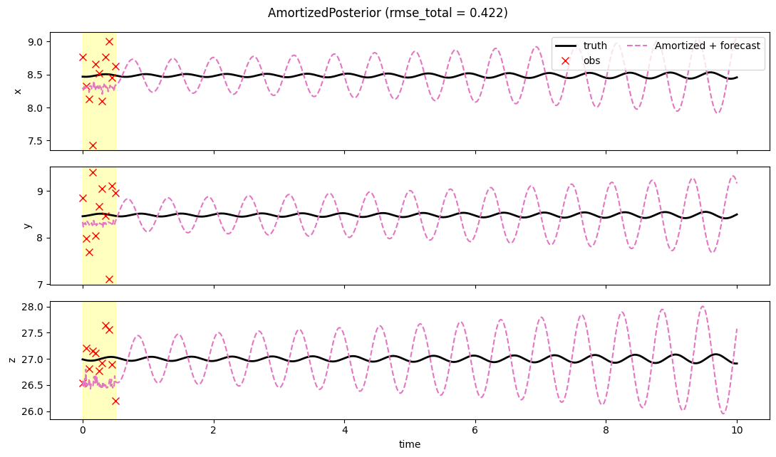

7. RMSE(t)¶

fig, ax = plt.subplots(figsize=(10, 3.5))
ax.axvspan(0.0, prob.T_assim * prob.dt, color="yellow", alpha=0.25)
ax.plot(t_axis, result.rmse_trace, "C6-", lw=2, label="Amortized")
ax.set_xlabel("time")
ax.set_ylabel("instantaneous RMSE")
ax.set_yscale("log")
ax.set_title("Amortized — analysis-then-forecast RMSE vs time")
ax.grid(True, alpha=0.3, which="both")
fig.tight_layout()
plt.show()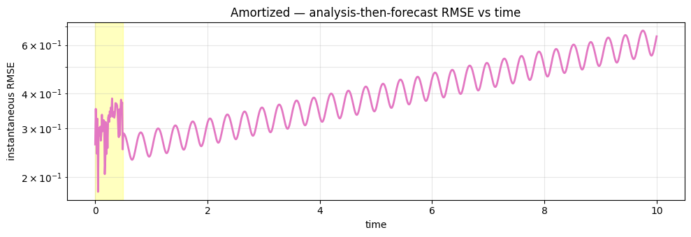

8. Discussion¶

Sub-millisecond MAP inference. The regression head learns the Lorenz attractor structure from simulated pairs, so for in- distribution problems the analysis is competitive with strong- 4DVar. The free-forecast (which uses the true L63 forward, not the network) then tracks the truth as long as the launch state was good.

Calibration caveat. Although the predictive mean tracks the truth, the NLL is large — the variances are mis-calibrated (typically too tight). This is the textbook amortized-inference failure mode and the reason for the six-step cycle gates (vardax.assert_posterior_agreement, vardax.simulation_based_calibration) — they catch “confident wrong answers” before they go operational.