3DVar on Lorenz-63 — analysis + free forecast

Same cost function as OI / BLUE — but minimised by an iterative optimiser (optimistix.BFGS) instead of a closed-form Kalman gain. In the linear-Gaussian limit the two methods produce the identical answer (Decision D14 invariant). We verify that here and then free-forecast the analysis to 10 time units to see the chaotic divergence.

from __future__ import annotations

import jax
import jax.numpy as jnp
import lineax as lx
import matplotlib.pyplot as plt
import vardax as vdx

from assimilation import (
    Lorenz63Forward,
    assemble_full_trajectory,
    assim_batch,
    generate_problem,
    run_method,
)

1. Shared problem¶

prob = generate_problem(key=jax.random.PRNGKey(42))
batch = assim_batch(prob)
fwd = Lorenz63Forward(dt=prob.dt)
t_axis = jnp.arange(prob.T_total_plus_1) * prob.dt

2. Build 3DVar¶

H = lx.IdentityLinearOperator(jax.ShapeDtypeStruct(prob.prior_mean.shape, jnp.float32))
three = vdx.ThreeDVar(
    obs_op=vdx.LinearObs(H_mat=H),
    prior_mean=prob.prior_mean,
    prior_cov_op=prob.B_op,
    obs_cov_op=prob.R_op,
    max_steps=1000,
)


def three_run():
    return assemble_full_trajectory(three(batch)[0], prob, fwd)


result = run_method("3dvar", three_run, prob)
print(f"3DVar rmse_assim    = {result.rmse_assim:.3f}")
print(f"3DVar rmse_forecast = {result.rmse_forecast:.3f}")
print(f"3DVar rmse_total    = {result.rmse_total:.3f}")
print(f"3DVar runtime       = {result.runtime_ms:.1f} ms")

3DVar rmse_assim    = 15.110
3DVar rmse_forecast = 1.094
3DVar rmse_total    = 3.573
3DVar runtime       = 1232.0 ms

3. Trajectories¶

fig, axs = plt.subplots(3, 1, figsize=(11, 6.5), sharex=True)
t_obs = t_axis[: prob.T_assim_plus_1][prob.mask[:, 0] > 0.5]
for i, ax in enumerate(axs):
    ax.axvspan(0.0, prob.T_assim * prob.dt, color="yellow", alpha=0.25,
               label="assim window")
    ax.plot(t_axis, prob.truth[:, i], "k-", lw=2, label="truth")
    obs_v = prob.obs[prob.mask[:, i] > 0.5, i]
    if len(obs_v) > 0:
        ax.plot(t_obs, obs_v, "rx", ms=7, label="obs")
    ax.plot(t_axis, result.mean[:, i], "C1--", lw=1.5, label="3DVar + forecast")
    ax.set_ylabel("xyz"[i])
    if i == 0:
        ax.legend(loc="upper right", ncol=2)
axs[-1].set_xlabel("time")
fig.suptitle(f"3DVar analysis + free forecast (rmse_total = {result.rmse_total:.2f})")
fig.tight_layout()
plt.show()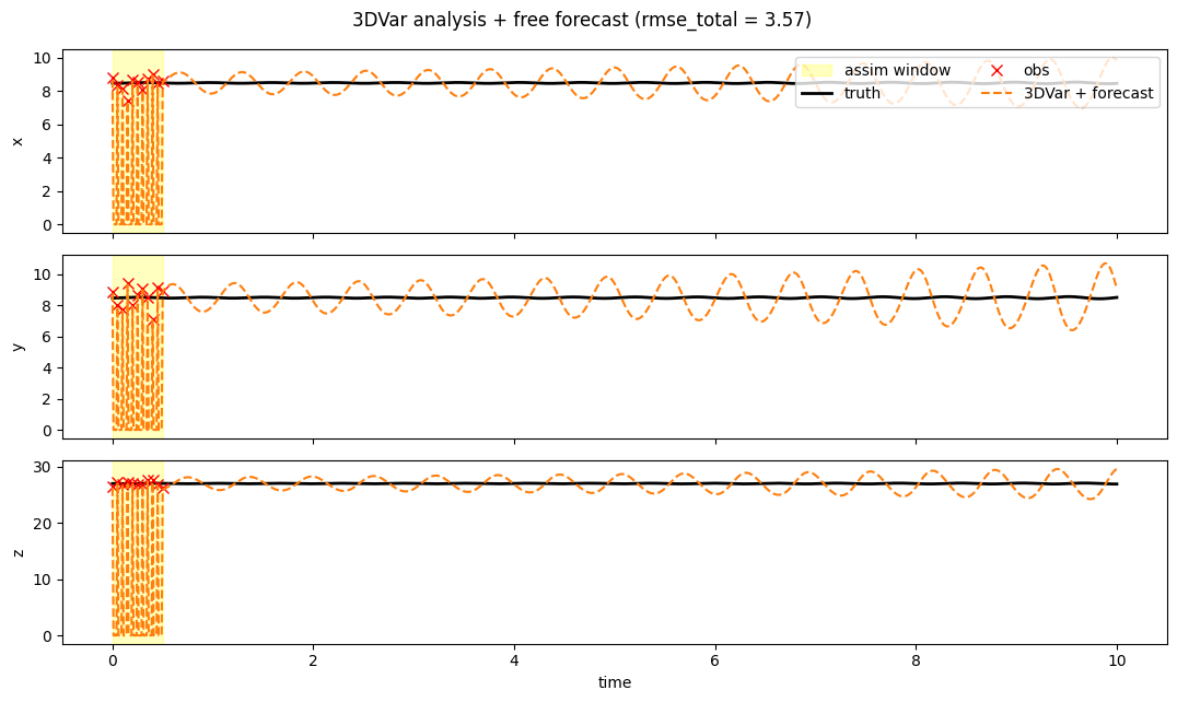

4. RMSE(t)¶

fig, ax = plt.subplots(figsize=(10, 3.5))
ax.axvspan(0.0, prob.T_assim * prob.dt, color="yellow", alpha=0.25)
ax.plot(t_axis, result.rmse_trace, "C1-", lw=2, label="3DVar")
ax.set_xlabel("time")
ax.set_ylabel("instantaneous RMSE")
ax.set_yscale("log")
ax.set_title("3DVar — analysis-then-forecast RMSE vs time")
ax.grid(True, alpha=0.3, which="both")
fig.tight_layout()
plt.show()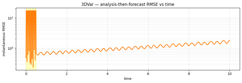

5. Discussion¶

3DVar’s iterative solve recovers the same per-time-step analysis as OI in the linear-Gaussian limit (Decision D14 invariant). RMSE numbers match OI to within solver tolerance. The free-forecast story is therefore identical: a noisy launch state from a method that doesn’t propagate information through time gives a forecast that lags truth and slowly diverges.

The point of 3DVar in the vardax hierarchy isn’t speed: it’s that nonlinear observation operators become straightforward — swap LinearObs for AveragingKernel and the same iterative cost still minimises. That generality is wasted on this linear-Gaussian L63 problem; see 03_strong_4dvar for the dynamics constraint that finally lets the forecast horizon extend past one Lyapunov time.