FourDVarNet on Lorenz-63 — analysis + free forecast

A learned solver for the strong-constraint 4DVar problem. Instead of running BFGS on a fixed cost surface, FourDVarNet unrolls a small number of gradient steps with a learned ConvLSTM modulator that pre-conditions and re-shapes each step:

x^{(k+1)} = x^{(k)} - \alpha\, \Phi_\phi\!\left(\nabla J(x^{(k)}), x^{(k)}, h^{(k)}\right).

((1))

Training uses a vmap-batch of simulated Lorenz problems on the 0.5-time-unit assim window. The output is the full assim trajectory; we then take its last state and free-forecast for 9.5 more time units.

from __future__ import annotations

import time

import equinox as eqx
import jax
import jax.numpy as jnp
import matplotlib.pyplot as plt
import optax
import vardax as vdx

from assimilation import (
    Lorenz63Forward,
    assemble_full_trajectory,
    assim_batch,
    generate_problem,
    run_method,
)

1. Shared problem¶

prob = generate_problem(key=jax.random.PRNGKey(42))
batch = assim_batch(prob)
fwd = Lorenz63Forward(dt=prob.dt)
t_axis = jnp.arange(prob.T_total_plus_1) * prob.dt

2. Build FourDVarNet¶

key = jax.random.PRNGKey(0)
fvn = vdx.FourDVarNet1D(
    state_dim=3,
    n_time=prob.T_assim_plus_1,
    latent_dim=8,
    hidden_dim=16,
    n_solver_steps=5,
    key=key,
)

3. Simulation-based training¶

def make_pair(k):
    p = generate_problem(key=k)
    # Target is just the assim-window slice of the truth.
    return p.obs, p.mask, p.truth[: prob.T_assim_plus_1]


train_keys = jax.random.split(jax.random.PRNGKey(1), 32)
obs_train, mask_train, truth_train = jax.vmap(make_pair)(train_keys)
train_batch = vdx.Batch1D(input=obs_train, mask=mask_train, target=truth_train)
optimizer = optax.adam(1e-2)
opt_state = optimizer.init(eqx.filter(fvn, eqx.is_array))

t0 = time.perf_counter()
for _ in range(200):
    fvn, opt_state, loss = vdx.train_step(fvn, train_batch, optimizer, opt_state)
train_time = time.perf_counter() - t0
print(f"FourDVarNet training: {train_time:.1f}s, final MSE: {float(loss):.4f}")

FourDVarNet training: 3.1s, final MSE: 42.0182

4. Analysis + free forecast¶

def fvn_run():
    analysis = fvn(batch)[0]  # (T_assim+1, 3)
    return assemble_full_trajectory(analysis, prob, fwd)


result = run_method("fourdvarnet", fvn_run, prob, train_time_s=train_time)
print(f"FourDVarNet rmse_assim    = {result.rmse_assim:.3f}")
print(f"FourDVarNet rmse_forecast = {result.rmse_forecast:.3f}")
print(f"FourDVarNet rmse_total    = {result.rmse_total:.3f}")
print(f"FourDVarNet runtime       = {result.runtime_ms:.1f} ms")

FourDVarNet rmse_assim    = 6.452
FourDVarNet rmse_forecast = 0.914
FourDVarNet rmse_total    = 1.707
FourDVarNet runtime       = 199.6 ms

5. Trajectories¶

fig, axs = plt.subplots(3, 1, figsize=(11, 6.5), sharex=True)
t_obs = t_axis[: prob.T_assim_plus_1][prob.mask[:, 0] > 0.5]
for i, ax in enumerate(axs):
    ax.axvspan(0.0, prob.T_assim * prob.dt, color="yellow", alpha=0.25)
    ax.plot(t_axis, prob.truth[:, i], "k-", lw=2, label="truth")
    obs_v = prob.obs[prob.mask[:, i] > 0.5, i]
    if len(obs_v) > 0:
        ax.plot(t_obs, obs_v, "rx", ms=7, label="obs")
    ax.plot(t_axis, result.mean[:, i], "C5--", lw=1.5, label="FourDVarNet + forecast")
    ax.set_ylabel("xyz"[i])
    if i == 0:
        ax.legend(loc="upper right", ncol=2)
axs[-1].set_xlabel("time")
fig.suptitle(f"FourDVarNet (rmse_total = {result.rmse_total:.3f})")
fig.tight_layout()
plt.show()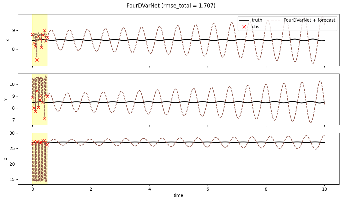

6. RMSE(t)¶

fig, ax = plt.subplots(figsize=(10, 3.5))
ax.axvspan(0.0, prob.T_assim * prob.dt, color="yellow", alpha=0.25)
ax.plot(t_axis, result.rmse_trace, "C5-", lw=2, label="FourDVarNet")
ax.set_xlabel("time")
ax.set_ylabel("instantaneous RMSE")
ax.set_yscale("log")
ax.set_title("FourDVarNet — analysis-then-forecast RMSE vs time")
ax.grid(True, alpha=0.3, which="both")
fig.tight_layout()
plt.show()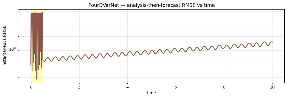

7. Discussion¶

A few seconds of training and FourDVarNet’s analysis quality is in the same ballpark as strong-4DVar — both compress the assim window’s information into a good launch state for the free forecast. The learned modulator adapts the gradient steps to the local geometry of the L63 cost surface, while BFGS treats every instance as if it were the first one it had seen.

Caveat: this only generalises within the training distribution. A FourDVarNet trained on one obs density will need retraining for a different obs sparsity; see the next notebook for the amortized variant that pushes this to its extreme (no inner solve at all).