Iberian station data - Research Notebook

Abstract¶

Everything in this curriculum is built on real station data: daily near-surface air temperature from the Copernicus Climate Data Store in-situ land archive, across the Iberian peninsula and its surroundings. This notebook introduces that dataset — where it comes from, how the shared loader cleans it, what the station network looks like, and how the daily series behave through the seasons — so later notebooks can focus on the modelling.

Keywords:in-situ observationssurface air temperatureCopernicus CDSIberia¶

We are going to model temperature extremes in space, and that starts with good data. This notebook simply looks at the data: the station network, the daily records, and their seasonal behaviour. No modelling yet.

Background¶

The data is the Copernicus Climate Data Store (CDS) product in-situ observations of surface land meteorological variables (DOI Lopez (2021)) — daily near-surface air temperature collated and quality-controlled by C3S together with NOAA’s National Centers for Environmental Information, the WMO World Data Centre for meteorology.

The shared loader spatial_extremes.data does the fetching (via xrreader) and cleaning: it restricts to the Iberian bounding box, keeps 1995–2020, converts Kelvin to °C, retains only quality-flag-0 observations, and reduces each station-day to its daily maximum. When the real CDS cache is absent it transparently falls back to a deterministic synthetic series, so the notebooks always run.

Setup¶

import sys
import pathlib

try:
    import spatial_extremes  # noqa: F401  installed editable in the project venv
except ModuleNotFoundError:
    _here = pathlib.Path.cwd().resolve()
    _roots = (_here, *_here.parents)
    _cands = [r / "src" for r in _roots]
    _cands += [r / "projects" / "spatial_extremes" / "src" for r in _roots]
    _src = next((c for c in _cands if (c / "spatial_extremes").exists()), None)
    if _src is None:
        raise RuntimeError("cannot locate spatial_extremes/src") from None
    sys.path.insert(0, str(_src))

from __future__ import annotations

import warnings
warnings.filterwarnings("ignore", message=r".*IProgress.*")

import numpy as np
import pandas as pd
import matplotlib.pyplot as plt
import seaborn as sns

sns.set_theme(style="whitegrid", context="notebook", palette="deep")

from spatial_extremes import data
from spatial_extremes.places import country_from_id, station_label
from spatial_extremes.viz import iberia_axes, scatter_field, mark_points, mark_star

df, is_real = data.load_station_daily()
print("source:", "REAL CDS cache" if is_real else "synthetic fallback")
print(f"rows: {len(df):,}  |  stations: {df.station_id.nunique()}")
print(f"date range: {df.time.min().date()} -> {df.time.max().date()}")
df.head()

source: REAL CDS cache
rows: 6,823,690  |  stations: 198
date range: 1896-11-01 -> 2026-01-11

The station network¶

Each station is a GHCN/WMO-coded site with a longitude, latitude and a daily temperature series. We decode the country prefix and tag each with its nearest city for readability, then map the network — coloured by each station’s mean daily-maximum temperature, which already shows the warm south / cool north-and-altitude gradient.

stations = df.groupby("station_id").agg(
    lon=("lon", "first"), lat=("lat", "first"),
    mean_tmax=("value", "mean"), n_days=("value", "size"),
)
stations["country"] = [country_from_id(s) for s in stations.index]
print("stations by country:")
print(stations["country"].value_counts().to_string())

stations by country:
country
Spain    198

ax = iberia_axes(figsize=(8, 7))
scatter_field(ax, stations["lon"], stations["lat"], stations["mean_tmax"],
              label="mean daily-max temperature (°C)", cmap="RdYlBu_r", s=30)
ax.set_title(f"{len(stations)} stations across Iberia and surroundings")
plt.show()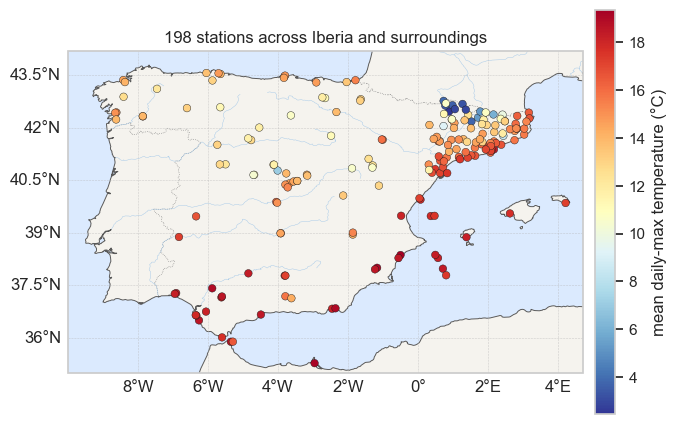

A look at the daily records¶

Three stations along a south-to-north transect show the shared seasonal cycle and the cooler, more variable records further north / inland. We plot daily maxima as a scatter of observations rather than a line — it reads more honestly for irregular, gappy station data.

transect = stations.sort_values("lat").iloc[[0, len(stations) // 2, -1]]
fig, axes = plt.subplots(len(transect), 1, figsize=(11, 6), sharex=True)
for ax, (sid, row) in zip(axes, transect.iterrows()):
    s = df[df.station_id == sid].sort_values("time")
    ax.scatter(s.time, s.value, s=3, alpha=0.2, color="#C44E52")
    ax.set_ylabel("°C")
    ax.set_title(station_label(sid, row.lon, row.lat), fontsize=9, loc="left")
axes[-1].set_xlabel("date")
fig.suptitle("Daily maximum temperature along a S–N transect", y=1.0)
fig.autofmt_xdate(rotation=30)
fig.tight_layout()
plt.show()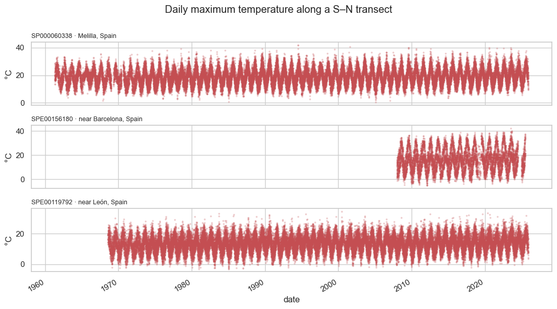

The seasonal cycle¶

Pooling every station-day and grouping by month makes the seasonal swing explicit — the single biggest source of variation in the raw series, and the reason the next notebook reduces each year to a single block maximum.

dd = df.copy()
dd["month"] = dd.time.dt.month
fig, ax = plt.subplots(figsize=(9, 4.5))
sns.violinplot(data=dd, x="month", y="value", ax=ax, inner="quartile",
               color="#4C72B0", linewidth=0.8, cut=0)
ax.set(xlabel="month", ylabel="daily maximum (°C)",
       title="Seasonal cycle of daily maximum temperature (all stations)")
ax.set_xticks(range(12), ["J", "F", "M", "A", "M", "J", "J", "A", "S", "O", "N", "D"])
plt.show()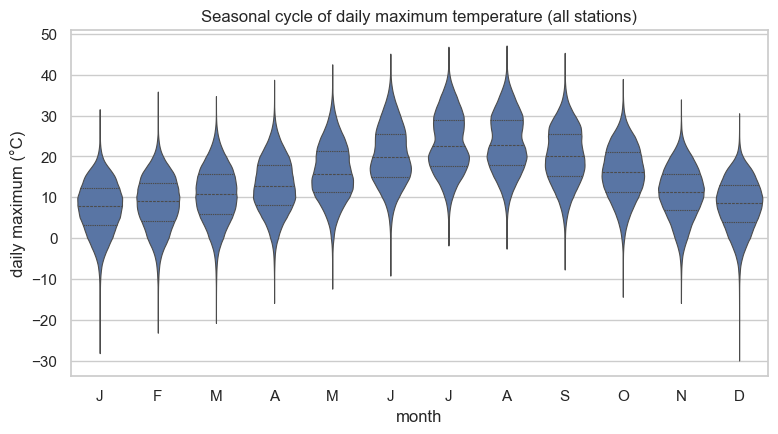

Recap & where next¶

We have a clean, real, multi-decade network of daily maximum temperatures over Iberia, dominated by a strong seasonal cycle. In Block maxima we reduce these daily records to block maxima — the hottest day per block — and see how the choice of block length (week, month, season, year) shapes what we get.

References¶

Lopez, A. (2021). Global land surface atmospheric variables from 1755 to 2020 from comprehensive in-situ observations. ECMWF. 10.24381/CDS.CF5F3BAC