Exact GP regression

Exact GP Regression — the Three Patterns¶

pyrox supports three modeling patterns for attaching priors to kernel hyperparameters. This notebook walks through all three using the collapsed Gaussian-likelihood path — same dataset, same SVI setup, same posterior — so the only thing that differs is how the priors are plumbed into the kernel.

What you’ll learn:

The fixed-hyperparameter GPPrior / ConditionedGP mechanics.
Three ways to attach priors to an RBF kernel — pure Equinox, PyroxModule, and Parameterized.
Fitting kernel hyperparameters with SVI via gp_factor.

Background¶

GP prior and likelihood¶

A Gaussian process prior with zero mean and covariance function $k_\theta$ places a joint Gaussian over any finite collection of function values: for inputs $X = \{x_i\}_{i=1}^N$ ,

p(f \mid X, \theta) = \mathcal{N}\!\bigl(f \mid 0, K_{XX}\bigr), \qquad (K_{XX})_{ij} = k_\theta(x_i, x_j).

((1))

With Gaussian observations $y_i = f(x_i) + \varepsilon_i$ and $\varepsilon_i \sim \mathcal{N}(0, \sigma^2)$ , the marginal likelihood is obtained by integrating out $f$ ,

p(y \mid X, \theta, \sigma^2) = \int p(y \mid f, \sigma^2)\, p(f \mid X, \theta)\, df = \mathcal{N}\!\bigl(y \mid 0, K_{XX} + \sigma^2 I\bigr).

((2))

Taking logs gives the collapsed log marginal likelihood that every GP regression workflow optimizes or samples:

\log p(y \mid X, \theta, \sigma^2) = -\tfrac{1}{2} y^\top (K_{XX} + \sigma^2 I)^{-1} y -\tfrac{1}{2}\log\bigl|K_{XX} + \sigma^2 I\bigr| -\tfrac{N}{2}\log(2\pi).

((3))

pyrox exposes this as gp_factor("obs", prior, y, noise_var), which delegates to gaussx.log_marginal_likelihood under the hood and drops into any NumPyro model.

Posterior predictive¶

Given training observations $(X, y)$ and test inputs $X_*$ , the GP posterior at $X_*$ is Gaussian with closed-form moments:

\mu_* = K_{*X}\bigl(K_{XX} + \sigma^2 I\bigr)^{-1} y,

((4))

\Sigma_* = K_{**} - K_{*X}\bigl(K_{XX} + \sigma^2 I\bigr)^{-1} K_{X*}.

((5))

GPPrior.condition(y, noise_var).predict(X_star) returns the diagonal of $\Sigma_*$ via gaussx.predict_mean and gaussx.predict_variance.

Kernel and hyperparameter priors¶

This notebook uses the squared-exponential (RBF) kernel,

k_\theta(x, x') = \sigma_f^2 \exp\!\Bigl(-\tfrac{\|x - x'\|^2}{2\ell^2}\Bigr), \qquad \theta = (\sigma_f^2, \ell),

((6))

with log-normal priors on both hyperparameters, $\sigma_f^2, \ell \sim \mathrm{LogNormal}(0, 1)$ . Log-normal keeps the samples positive without the explicit dist.constraints.positive bookkeeping that Parameterized handles automatically for pattern C.

The three patterns¶

Pattern	Where hyperparameters live	When to reach for it
A	Pure `eqx.Module`, sampled in the NumPyro model, spliced with `eqx.tree_at`	Lightweight; drop a Bayesian layer into existing Equinox code.
B	Custom `PyroxModule` kernel, sampled inside `__call__` via `pyrox_sample`	Self-contained probabilistic kernel; no model-side plumbing.
C	`Parameterized` kernel (pyrox ships `RBF`, `Matern`, etc.); `set_prior` / `autoguide` / `set_mode`	Rich registry with constraints, priors, and mode switching.

All three fit the same data to the same posterior — the choice is ergonomics.

Setup¶

Detect Colab and install pyrox[colab] (which pulls in matplotlib and watermark) only when running there. Local / CI users with the environment already set up skip the install and go straight to the imports.

import subprocess
import sys


try:
    import google.colab  # noqa: F401

    IN_COLAB = True
except ImportError:
    IN_COLAB = False

if IN_COLAB:
    subprocess.run(
        [
            sys.executable,
            "-m",
            "pip",
            "install",
            "-q",
            "pyrox[colab] @ git+https://github.com/jejjohnson/pyrox@main",
        ],
        check=True,
    )

import warnings


warnings.filterwarnings("ignore", message=r".*IProgress.*")

import equinox as eqx
import jax
import jax.numpy as jnp
import jax.random as jr
import matplotlib.pyplot as plt
import numpyro
import numpyro.distributions as dist
from jaxtyping import Array, Float
from numpyro.infer import SVI, Trace_ELBO
from numpyro.infer.autoguide import AutoNormal
from numpyro.optim import Adam

from pyrox._core import PyroxModule, pyrox_method
from pyrox.gp import RBF, GPPrior, Kernel, gp_factor
from pyrox.gp._src.kernels import rbf_kernel


jax.config.update("jax_enable_x64", True)

Print an explicit version / platform readout so reproducing this notebook later is unambiguous.

import importlib.util


try:
    from IPython import get_ipython

    ipython = get_ipython()
except ImportError:
    ipython = None

if ipython is not None and importlib.util.find_spec("watermark") is not None:
    ipython.run_line_magic("load_ext", "watermark")
    ipython.run_line_magic(
        "watermark",
        "-v -m -p jax,equinox,numpyro,gaussx,pyrox,matplotlib",
    )
else:
    print("watermark extension not installed; skipping reproducibility readout.")

Python implementation: CPython
Python version       : 3.12.13
IPython version      : 9.12.0

jax       : 0.8.3
equinox   : 0.13.7
numpyro   : 0.20.1
gaussx    : 0.0.10
pyrox     : 0.0.6
matplotlib: 3.10.8

Compiler    : GCC 14.3.0
OS          : Linux
Release     : 6.8.0-1044-azure
Machine     : x86_64
Processor   : x86_64
CPU cores   : 16
Architecture: 64bit

Toy dataset¶

A noisy sine curve with a gap — the gap is where the posterior uncertainty band should visibly widen for any well-fit GP.

key = jr.PRNGKey(0)

f_true = lambda x: jnp.sin(2.0 * x) + 0.3 * jnp.cos(5.0 * x)

X_train = jnp.concatenate(
    [jnp.linspace(-3.0, -0.5, 10), jnp.linspace(1.5, 3.0, 10)]
).reshape(-1, 1)
noise_std = 0.15
y_train = f_true(X_train.squeeze(-1)) + noise_std * jr.normal(key, (X_train.shape[0],))
X_test = jnp.linspace(-3.5, 3.5, 200).reshape(-1, 1)
noise_var = jnp.array(noise_std**2)

print(f"Training points: {X_train.shape[0]}")
print(f"Test points:     {X_test.shape[0]}")

Training points: 20
Test points:     200

Fixed-hyperparameter baseline¶

Before looking at priors, it’s useful to see the raw mechanics of the GPPrior / ConditionedGP path. Instantiate an RBF with default hyperparameters, condition on the observations, predict on a dense grid. GPPrior.solver defaults to gaussx.DenseSolver(); swap for any other gaussx.AbstractSolverStrategy at construction time.

kernel_fixed = RBF(init_variance=1.0, init_lengthscale=0.6)
prior_fixed = GPPrior(kernel=kernel_fixed, X=X_train)

with numpyro.handlers.seed(rng_seed=0):
    cond_fixed = prior_fixed.condition(y_train, noise_var)
    mean_fixed, var_fixed = cond_fixed.predict(X_test)
std_fixed = jnp.sqrt(jnp.clip(var_fixed, min=0.0))


def plot_posterior(ax, mean, std, label):
    ax.plot(
        X_test.squeeze(),
        f_true(X_test.squeeze()),
        "k--",
        lw=1.5,
        label="True function",
        zorder=4,
    )
    ax.plot(X_test.squeeze(), mean, "C0-", lw=2, label=f"{label} mean", zorder=3)
    ax.fill_between(
        X_test.squeeze(),
        mean - 2 * std,
        mean + 2 * std,
        color="C0",
        alpha=0.2,
        label=r"$\pm 2\sigma$",
    )
    ax.scatter(
        X_train.squeeze(),
        y_train,
        s=30,
        c="C1",
        edgecolors="k",
        linewidths=0.5,
        label="Training data",
        zorder=5,
    )
    ax.set_xlabel("x")
    ax.set_ylabel("y")
    ax.legend(loc="lower left", fontsize=9)


fig, ax = plt.subplots(figsize=(12, 5))
plot_posterior(ax, mean_fixed, std_fixed, "Fixed-hyperparameter")
ax.set_title("GP posterior with fixed RBF hyperparameters")
plt.show()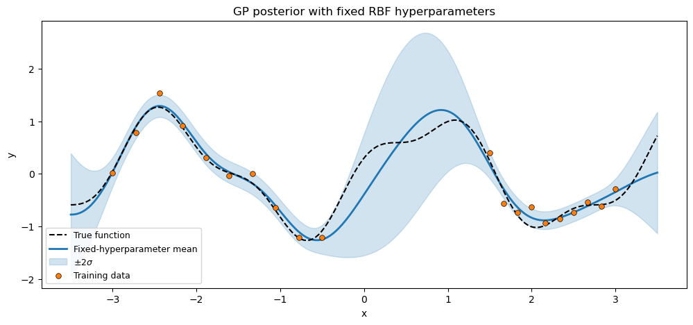

Now we turn the RBF’s variance and lengthscale into random variables with $\mathrm{LogNormal}(0, 1)$ priors, and fit them with SVI. The three patterns differ only in how the priors are attached to the kernel — the NumPyro model, SVI loop, and final posterior are the same.

Fitting hyperparameters with SVI¶

Stochastic variational inference maximizes the ELBO

\mathcal{L}(q) = \mathbb{E}_{q(\theta)}\bigl[\log p(y, \theta)\bigr] - \mathbb{E}_{q(\theta)}\bigl[\log q(\theta)\bigr] = \mathbb{E}_{q(\theta)}\bigl[\log p(y \mid \theta)\bigr] - \mathrm{KL}\!\bigl(q(\theta) \,\|\, p(\theta)\bigr),

((7))

where $q(\theta)$ is the variational family — here AutoNormal which places a mean-field Gaussian on each transformed hyperparameter. The three patterns differ only in how the prior $p(\theta)$ is attached to the kernel.

Pattern A — pure Equinox + `eqx.tree_at`¶

Write a minimal Kernel subclass with variance and lengthscale as plain eqx.Module fields. Sample the hyperparameters inside the NumPyro model and splice them into the kernel with eqx.tree_at.

\theta \sim p(\theta) \;\Rightarrow\; k = \text{tree\_at}(k_0, \theta) \;\Rightarrow\; \log p(y \mid X, \theta) \text{ via gp\_factor}.

((8))

Use this when you already have Equinox-native modules and want to add priors without subclassing any pyrox machinery.

class RBFLite(Kernel):
    """Minimal Equinox-native RBF kernel."""

    variance: Float[Array, ""]
    lengthscale: Float[Array, ""]

    def __call__(
        self, X1: Float[Array, "N1 D"], X2: Float[Array, "N2 D"]
    ) -> Float[Array, "N1 N2"]:
        return rbf_kernel(X1, X2, self.variance, self.lengthscale)


def model_pattern_a(X, y, noise_var):
    variance = numpyro.sample("variance", dist.LogNormal(0.0, 1.0))
    lengthscale = numpyro.sample("lengthscale", dist.LogNormal(0.0, 1.0))
    kernel = RBFLite(variance=jnp.array(1.0), lengthscale=jnp.array(1.0))
    kernel = eqx.tree_at(
        lambda k: (k.variance, k.lengthscale),
        kernel,
        (variance, lengthscale),
    )
    prior = GPPrior(kernel=kernel, X=X)
    gp_factor("obs", prior, y, noise_var)

Pattern B — `PyroxModule` kernel with `pyrox_sample`¶

Subclass PyroxModule (and Kernel for the protocol) and register the hyperparameters as sample sites inside __call__ via self.pyrox_sample. The pyrox_method decorator activates the per-call cache so every kernel(X1, X2) invocation sees the same hyperparameter draw:

k(x, x') = \sigma_f^2 \exp\!\bigl(-\|x-x'\|^2 / 2\ell^2\bigr), \quad \sigma_f^2, \ell \sim p(\theta) \text{ on first call}.

((9))

The kernel now owns its probabilistic semantics — the NumPyro model doesn’t need to plumb anything.

class RBFPyrox(Kernel, PyroxModule):
    """PyroxModule kernel with inline prior registration."""

    pyrox_name: str = "RBFPyrox"

    @pyrox_method
    def __call__(
        self, X1: Float[Array, "N1 D"], X2: Float[Array, "N2 D"]
    ) -> Float[Array, "N1 N2"]:
        variance = self.pyrox_sample("variance", dist.LogNormal(0.0, 1.0))
        lengthscale = self.pyrox_sample("lengthscale", dist.LogNormal(0.0, 1.0))
        return rbf_kernel(X1, X2, variance, lengthscale)


def model_pattern_b(X, y, noise_var):
    kernel = RBFPyrox()
    prior = GPPrior(kernel=kernel, X=X)
    gp_factor("obs", prior, y, noise_var)

Pattern C — `Parameterized` kernel with `set_prior`¶

Use the shipped pyrox.gp.RBF class and call set_prior once per hyperparameter. Parameterized owns the registry: priors, guides (autoguide), constraints, and mode switching all live here.

Because variance and lengthscale were registered with the positivity constraint on the Parameterized side, the $\mathrm{LogNormal}(0, 1)$ prior composes cleanly through a TransformedDistribution,

q(\theta) = \mathrm{biject}\bigl(\mathcal{N}\!\bigl(\mu_\theta, \mathrm{diag}(\sigma_\theta^2)\bigr)\bigr),

((10))

so every SVI draw is guaranteed to land in the prior’s support.

This is the richest of the three patterns — reach for it when you want the full priors / autoguide / mode story without hand-rolling it.

def model_pattern_c(X, y, noise_var):
    kernel = RBF()
    kernel.set_prior("variance", dist.LogNormal(0.0, 1.0))
    kernel.set_prior("lengthscale", dist.LogNormal(0.0, 1.0))
    prior = GPPrior(kernel=kernel, X=X)
    gp_factor("obs", prior, y, noise_var)

Fit all three with the same SVI loop¶

def fit(model_fn, seed, n_steps=400):
    guide = AutoNormal(model_fn)
    svi = SVI(model_fn, guide, Adam(5e-2), Trace_ELBO())
    state = svi.init(jr.PRNGKey(seed), X_train, y_train, noise_var)
    losses = []
    for _ in range(n_steps):
        state, loss = svi.update(state, X_train, y_train, noise_var)
        losses.append(float(loss))
    return state, svi, losses


state_a, svi_a, losses_a = fit(model_pattern_a, 1)
state_b, svi_b, losses_b = fit(model_pattern_b, 2)
state_c, svi_c, losses_c = fit(model_pattern_c, 3)


def posterior_hyperparams(svi, state, variance_site, lengthscale_site):
    params = svi.get_params(state)
    variance = float(jnp.exp(params[f"{variance_site}_auto_loc"]))
    lengthscale = float(jnp.exp(params[f"{lengthscale_site}_auto_loc"]))
    return variance, lengthscale


v_a, ls_a = posterior_hyperparams(svi_a, state_a, "variance", "lengthscale")
v_b, ls_b = posterior_hyperparams(
    svi_b, state_b, "RBFPyrox.variance", "RBFPyrox.lengthscale"
)
v_c, ls_c = posterior_hyperparams(svi_c, state_c, "RBF.variance", "RBF.lengthscale")

print(f"{'pattern':<10} {'variance':>10} {'lengthscale':>12}")
print("-" * 36)
print(f"{'A':<10} {v_a:>10.3f} {ls_a:>12.3f}")
print(f"{'B':<10} {v_b:>10.3f} {ls_b:>12.3f}")
print(f"{'C':<10} {v_c:>10.3f} {ls_c:>12.3f}")

pattern      variance  lengthscale
------------------------------------
A               0.825        0.439
B               0.617        0.451
C               0.792        0.429

The three fitted posteriors should agree up to stochastic SVI noise — a good sanity check that the patterns are semantically equivalent.

fig, ax = plt.subplots(figsize=(12, 5))
ax.plot(losses_a, "C0-", label="Pattern A", alpha=0.85)
ax.plot(losses_b, "C1-", label="Pattern B", alpha=0.85)
ax.plot(losses_c, "C2-", label="Pattern C", alpha=0.85)
ax.set_xlabel("SVI step")
ax.set_ylabel(r"$-$ELBO")
ax.set_title("SVI convergence — three patterns")
ax.legend()
plt.show()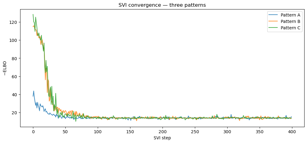

Rebuild each kernel at the fitted posterior mean and predict on the dense grid. Overlaying the three posterior means makes it easy to confirm they agree.

def predict_with(variance, lengthscale):
    kernel = RBF(init_variance=variance, init_lengthscale=lengthscale)
    prior = GPPrior(kernel=kernel, X=X_train)
    with numpyro.handlers.seed(rng_seed=0):
        cond = prior.condition(y_train, noise_var)
        mean, var = cond.predict(X_test)
    return mean, jnp.sqrt(jnp.clip(var, min=0.0))


mean_a, std_a = predict_with(v_a, ls_a)
mean_b, std_b = predict_with(v_b, ls_b)
mean_c, std_c = predict_with(v_c, ls_c)

fig, axes = plt.subplots(1, 3, figsize=(18, 5), sharey=True)
for ax, mean, std, title in zip(
    axes,
    [mean_a, mean_b, mean_c],
    [std_a, std_b, std_c],
    ["Pattern A", "Pattern B", "Pattern C"],
):
    plot_posterior(ax, mean, std, title)
    ax.set_title(title)
plt.tight_layout()
plt.show()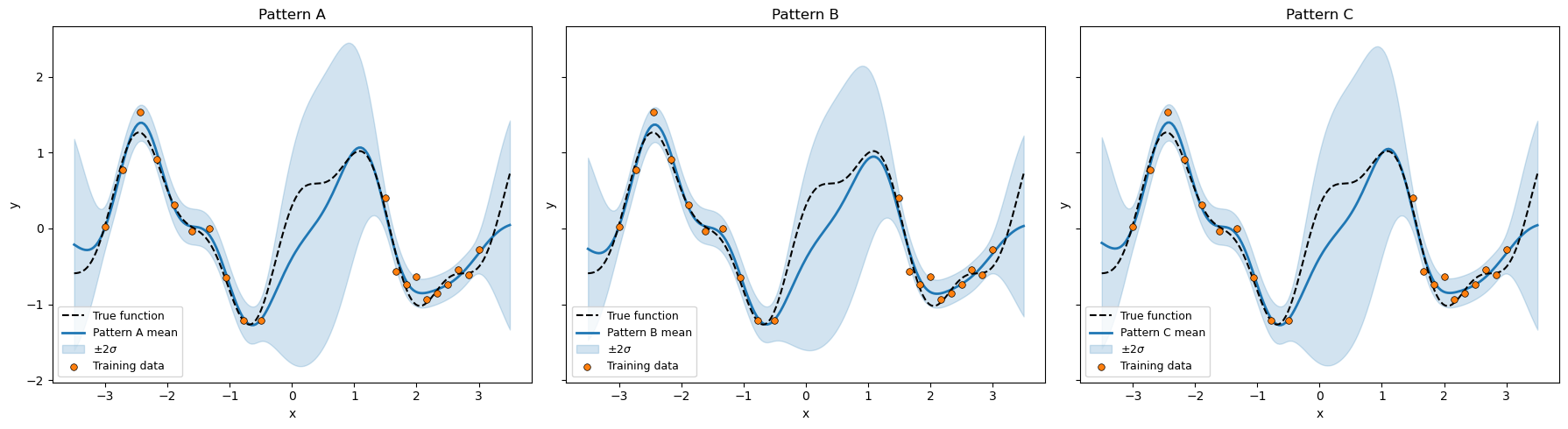

When to use which¶

Pattern A — lightest touch. Good when the rest of your code is already pure Equinox and you want to sprinkle a single Bayesian layer on top. No pyrox base classes needed.
Pattern B — the kernel is probabilistic by construction. Good when you ship a reusable kernel and want the priors to travel with it. Pick this when the kernel is genuinely “one thing” that happens to have randomness.
Pattern C — full registry. Best when you want constraints, autoguides, mode switching, and the rich set_prior / autoguide / set_mode API. The shipped RBF, Matern, Periodic, etc. use this pattern; subclass Parameterized for your own.

All three compose with NumPyro handlers, MCMC, SVI, and JAX transforms identically — the choice is purely ergonomic.