Borrowing strength across stations

Abstract¶

Independent fits waste information; complete pooling throws away real variation. A hierarchical GEV is the principled middle: each station keeps its own parameters, tied by a shared prior whose spread τ is learned from the data. Fit with a non-centred NUTS parameterisation, the model pools each parameter exactly as much as the data warrant — leaving the location μ free while collapsing the noisy tail ξ onto a single shared value, and cutting the 100-year-level uncertainty sharply. Its one blind spot, that the pooling is spatially agnostic, sets up the Gaussian-process field to come.

Keywords:partial poolinghierarchical modelshrinkagenon-centred parameterisationNeal's funnelreturn levels¶

Notebook 04 fit every station on its own and found the tails ξ — and the 100-year levels that lean on them — were dominated by sampling noise: a few decades of annual maxima cannot pin down a tail. The opposite extreme, complete pooling, would force a single ξ on all stations, throwing away any real geographic variation. Partial pooling is the principled middle ground: a hierarchical model in which each station keeps its own parameters, but they are tied together by a shared prior whose spread is learned from the data.

We keep the GEV likelihood and the stabilising reparameterisation from notebook 04 ( $\log\sigma$ , $\xi = \tfrac12\tanh\tilde\xi$ ), and add a group level on top of each parameter:

\begin{aligned} \mu_s &\sim \mathcal N(\mu_0,\ \tau_\mu^2), & \log\sigma_s &\sim \mathcal N(\lambda_0,\ \tau_\lambda^2), & \tilde\xi_s &\sim \mathcal N(\xi_0,\ \tau_\xi^2), \end{aligned}

((1))

with weak hyperpriors on the group means $(\mu_0, \lambda_0, \xi_0)$ and group spreads $(\tau_\mu, \tau_\lambda, \tau_\xi)$ . The likelihood is unchanged: $y_{s,t} \sim \mathrm{GEV}(\mu_s, \sigma_s, \xi_s)$ .

All the action is in the τ’s, which control how hard each parameter is pooled:

if the stations genuinely differ, the data push τ large and partial pooling $\to$ no pooling;
if they don’t, the data pull $\tau \to 0$ and partial pooling $\to$ complete pooling.

The model decides this per parameter, automatically. We will watch μ stay free while ξ collapses onto a single shared tail — precisely because notebook 04 already showed μ carries signal and ξ carries almost none.

import sys
import pathlib

try:
    import spatial_extremes  # noqa: F401  installed editable in the project venv
except ModuleNotFoundError:
    _here = pathlib.Path.cwd().resolve()
    _roots = (_here, *_here.parents)
    _cands = [r / "src" for r in _roots]
    _cands += [r / "projects" / "spatial_extremes" / "src" for r in _roots]
    _src = next((c for c in _cands if (c / "spatial_extremes").exists()), None)
    if _src is None:
        raise RuntimeError("cannot locate spatial_extremes/src") from None
    sys.path.insert(0, str(_src))

import jax
jax.config.update("jax_enable_x64", True)

import time

import numpy as np
import jax
import jax.numpy as jnp
import jax.random as jr
import matplotlib.pyplot as plt

import numpyro
import numpyro.distributions as ndist
from numpyro.infer import MCMC, NUTS
from numpyro.infer.initialization import init_to_median

from xtremax import GeneralizedExtremeValueDistribution as GEV
from spatial_extremes import data
from spatial_extremes.viz import iberia_axes, scatter_field

maxima, stations, years, is_real = data.load_annual_maxima(min_years=20)
Y = jnp.asarray(maxima)              # (S, T) — NaN where a station-year is missing
mask = ~jnp.isnan(Y)                 # observed-entry mask for the likelihood
lon, lat = stations[:, 0], stations[:, 1]
S, T = Y.shape
ybar = jnp.asarray(np.nanmean(maxima, axis=1))
ystd = jnp.asarray(np.nanstd(maxima, axis=1))
print("source:", "REAL" if is_real else "SYNTHETIC",
      "| stations", S, "| years", f"{years.min()}-{years.max()}", f"({T})")
print(f"coverage: {int(np.asarray(mask.sum(1)).min())}-"
      f"{int(np.asarray(mask.sum(1)).max())} yrs/station, "
      f"{100 * float(mask.mean()):.0f}% of the {S}×{T} grid observed")


def summarise(post, name):
    a = post[name]
    return (np.asarray(jnp.median(a, 0)),
            np.asarray(jnp.quantile(a, 0.025, 0)),
            np.asarray(jnp.quantile(a, 0.975, 0)))

/Users/eman/code_projects/research_notebook/projects/spatial_extremes/.venv/lib/python3.12/site-packages/tqdm/auto.py:21: TqdmWarning: IProgress not found. Please update jupyter and ipywidgets. See https://ipywidgets.readthedocs.io/en/stable/user_install.html
  from .autonotebook import tqdm as notebook_tqdm

source: REAL | stations 107 | years 1897-2025 (125)
coverage: 23-120 yrs/station, 49% of the 107×125 grid observed

The no-pooling baseline (recap)¶

First we re-fit the independent model from notebook 04 — the stabilised parameterisation, each station on its own — to have something to pool against.

def gev_no_pool(Y):
    with numpyro.plate("stations", S):
        mu = numpyro.sample("mu", ndist.Normal(ybar, 5.0))
        log_sigma = numpyro.sample("log_sigma", ndist.Normal(jnp.log(ystd), 0.5))
        xi_t = numpyro.sample("xi_t", ndist.Normal(0.0, 0.5))
        sigma = numpyro.deterministic("sigma", jnp.exp(log_sigma))
        xi = numpyro.deterministic("xi", 0.5 * jnp.tanh(xi_t))
    yf = jnp.where(mask, Y, ybar[:, None])     # masked likelihood (ragged records)
    lp = GEV(loc=mu[:, None], scale=sigma[:, None],
             concentration=xi[:, None]).log_prob(yf)
    numpyro.factor("obs", jnp.where(mask, lp, 0.0).sum())

mcmc_np = MCMC(NUTS(gev_no_pool, init_strategy=init_to_median,
                    target_accept_prob=0.99),
               num_warmup=1500, num_samples=1000, num_chains=1, progress_bar=False)
t0 = time.time()
mcmc_np.run(jr.PRNGKey(0), Y, extra_fields=("diverging",))
np_post = mcmc_np.get_samples()
print(f"no-pool: {time.time() - t0:.1f}s · "
      f"{int(mcmc_np.get_extra_fields()['diverging'].sum())} divergences")
np_mu, _, _ = summarise(np_post, "mu")
np_sig, _, _ = summarise(np_post, "sigma")
np_xi, np_xi_lo, np_xi_hi = summarise(np_post, "xi")

no-pool: 3.0s · 49 divergences

The hierarchical model¶

Two practical points make this sample cleanly:

Non-centred parameterisation. Writing $\mu_s = \mu_0 + \tau_\mu\, z_s$ with $z_s \sim \mathcal N(0,1)$ (and likewise for the others) decouples each station from the group spread it lives in. The centred form $\mu_s \sim \mathcal N(\mu_0, \tau_\mu^2)$ creates Neal’s funnel — a pinched geometry that diverges as $\tau \to 0$ , exactly the regime we expect for ξ. The non-centred form is mathematically identical but funnel-free.
The same $\log\sigma$ / bounded-ξ tricks from notebook 04 keep us off the GEV support edge.

So the latent draws are the standardised $z$ ’s and the six hyperparameters; the per-station $(\mu_s, \sigma_s, \xi_s)$ are deterministic transforms.

gmean = float(np.nanmean(maxima))
log_sd0 = float(np.log(np.nanmean(np.nanstd(maxima, axis=1))))

def gev_hier(Y):
    # group level (hyperparameters)
    mu0 = numpyro.sample("mu0", ndist.Normal(gmean, 10.0))
    tau_mu = numpyro.sample("tau_mu", ndist.HalfNormal(5.0))
    lam0 = numpyro.sample("lam0", ndist.Normal(log_sd0, 0.5))
    tau_lam = numpyro.sample("tau_lam", ndist.HalfNormal(0.5))
    xi0 = numpyro.sample("xi0", ndist.Normal(0.0, 0.3))
    tau_xi = numpyro.sample("tau_xi", ndist.HalfNormal(0.3))
    # station level (non-centred)
    with numpyro.plate("stations", S):
        z_mu = numpyro.sample("z_mu", ndist.Normal(0.0, 1.0))
        z_lam = numpyro.sample("z_lam", ndist.Normal(0.0, 1.0))
        z_xi = numpyro.sample("z_xi", ndist.Normal(0.0, 1.0))
        mu = numpyro.deterministic("mu", mu0 + tau_mu * z_mu)
        sigma = numpyro.deterministic("sigma", jnp.exp(lam0 + tau_lam * z_lam))
        xi = numpyro.deterministic("xi", 0.5 * jnp.tanh(xi0 + tau_xi * z_xi))
    yf = jnp.where(mask, Y, ybar[:, None])     # masked likelihood (ragged records)
    lp = GEV(loc=mu[:, None], scale=sigma[:, None],
             concentration=xi[:, None]).log_prob(yf)
    numpyro.factor("obs", jnp.where(mask, lp, 0.0).sum())

mcmc_h = MCMC(NUTS(gev_hier, init_strategy=init_to_median, target_accept_prob=0.95),
              num_warmup=1500, num_samples=1000, num_chains=1, progress_bar=False)
t0 = time.time()
mcmc_h.run(jr.PRNGKey(0), Y, extra_fields=("diverging",))
h_post = mcmc_h.get_samples()
print(f"hierarchical: {time.time() - t0:.1f}s · "
      f"{int(mcmc_h.get_extra_fields()['diverging'].sum())} divergences")
h_mu, h_mu_lo, h_mu_hi = summarise(h_post, "mu")
h_sig, _, _ = summarise(h_post, "sigma")
h_xi, h_xi_lo, h_xi_hi = summarise(h_post, "xi")

hierarchical: 1.6s · 10 divergences

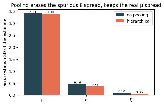
How hard did each parameter pool?¶

The learned group spread τ is the dial. Compare it with the across-station spread of the no-pool estimates: when τ is large the stations are allowed to differ; when $\tau \approx 0$ the model has concluded they don’t, and pulls every station onto the shared value.

for name in ["tau_mu", "tau_lam", "tau_xi"]:
    q = np.quantile(np.asarray(h_post[name]), [0.025, 0.5, 0.975])
    print(f"{name:8s} posterior median {q[1]:.3f}  (95% CI {q[0]:.3f}–{q[2]:.3f})")

fig, ax = plt.subplots(figsize=(6.0, 3.8))
labels = ["μ", "σ", "ξ"]
np_sd = [np_mu.std(), np_sig.std(), np_xi.std()]
h_sd = [h_mu.std(), h_sig.std(), h_xi.std()]
x = np.arange(3)
ax.bar(x - 0.2, np_sd, 0.4, label="no pooling", color="#264653")
ax.bar(x + 0.2, h_sd, 0.4, label="hierarchical", color="#e76f51")
ax.set_xticks(x)
ax.set_xticklabels(labels)
ax.set_ylabel("across-station SD of the estimate")
ax.set_title("Pooling erases the spurious ξ spread, keeps the real μ spread")
ax.legend()
for xi_, a, b in zip(x, np_sd, h_sd):
    ax.text(xi_ - 0.2, a, f"{a:.2f}", ha="center", va="bottom", fontsize=8)
    ax.text(xi_ + 0.2, b, f"{b:.2f}", ha="center", va="bottom", fontsize=8)
plt.show()

tau_mu   posterior median 3.393  (95% CI 2.941–3.923)
tau_lam  posterior median 0.200  (95% CI 0.169–0.237)
tau_xi   posterior median 0.228  (95% CI 0.169–0.292)

Shrinkage in action¶

The classic hierarchical picture: each station’s estimate is pulled from its lonely no-pool value toward the group. The distance it travels is the shrinkage, and it is set by how little that station’s data had to say. For μ the lines are nearly flat — the data win. For ξ they sweep together onto a single shared tail — the group wins.

fig, axes = plt.subplots(1, 2, figsize=(11, 4.8))
for ax, npv, hv, ylab, ttl in [
    (axes[0], np_mu, h_mu, "μ  location (°C)", "μ barely moves — the data win"),
    (axes[1], np_xi, h_xi, "ξ  shape", "ξ collapses onto one shared tail"),
]:
    for i in range(S):
        ax.plot([0, 1], [npv[i], hv[i]], color="0.65", lw=0.5, alpha=0.6,
                zorder=1)
    ax.scatter(np.zeros(S), npv, s=14, color="#264653", zorder=3,
               label="no pooling")
    ax.scatter(np.ones(S), hv, s=14, color="#e76f51", zorder=3,
               label="hierarchical")
    ax.axhline(hv.mean(), 0.5, 1.0, ls="--", color="0.4", lw=0.8)
    ax.set_xlim(-0.25, 1.25)
    ax.set_xticks([0, 1])
    ax.set_xticklabels(["no pool", "hierarchical"])
    ax.set_ylabel(ylab)
    ax.set_title(ttl)
    ax.legend(fontsize=8, loc="best")
plt.show()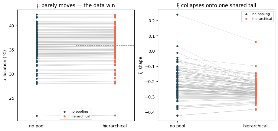

The pooled maps¶

Side by side with notebook 04: μ is essentially unchanged (it never needed help), while the ξ map has gone from noisy static to a near-uniform field — the model’s verdict that the tails are, to the resolution the data allow, the same everywhere.

try:
    import cartopy.crs as ccrs
    proj = {"projection": ccrs.PlateCarree()}
except Exception:
    proj = {}

fig, axs = plt.subplots(2, 2, figsize=(12.5, 9.5), subplot_kw=proj)
for j, (np_v, h_v, label, cmap) in enumerate([
    (np_mu, h_mu, "μ̂  location (°C)", "RdYlBu_r"),
    (np_xi, h_xi, "ξ̂  shape", "plasma"),
]):
    vmin = min(np_v.min(), h_v.min())
    vmax = max(np_v.max(), h_v.max())
    for k, (vals, tag) in enumerate([(np_v, "no pooling"), (h_v, "hierarchical")]):
        ax = iberia_axes(ax=axs[j, k])
        scatter_field(ax, lon, lat, vals, label=label, cmap=cmap,
                      vmin=vmin, vmax=vmax)
        ax.set_title(f"{tag} · {label}")
plt.show()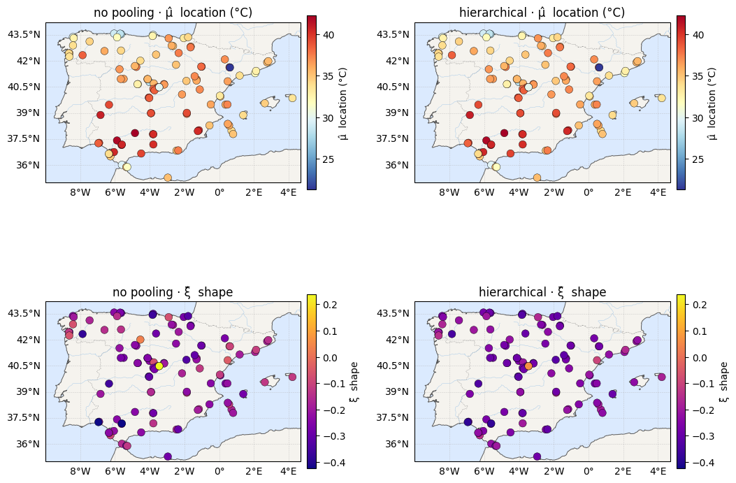

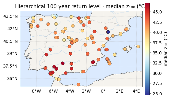
What the planner gets¶

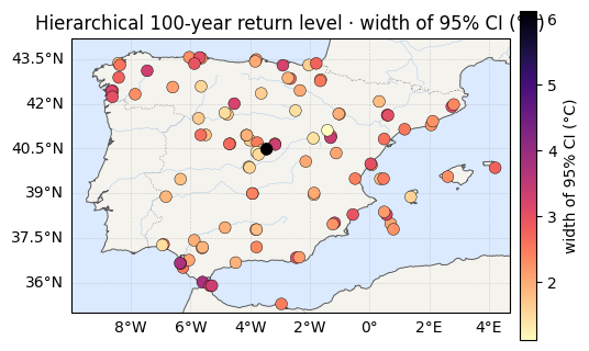
The 100-year return level inherits the pooled tail. Compared with the no-pooling fit, the $z_{100}$ map is smoother and — more importantly — its credible intervals shrink, because each station now borrows tail information from all the others instead of guessing from its own short record.

def rl100(post):
    RL = GEV(loc=post["mu"], scale=post["sigma"],
             concentration=post["xi"]).return_level(100.0)
    return (np.asarray(jnp.median(RL, 0)),
            np.asarray(jnp.quantile(RL, 0.975, 0) - jnp.quantile(RL, 0.025, 0)))

np_rl, np_rlw = rl100(np_post)
h_rl, h_rlw = rl100(h_post)
print(f"z100 95% CI width — no pooling : {np_rlw.mean():.1f} °C avg "
      f"(max {np_rlw.max():.1f})")
print(f"z100 95% CI width — hierarchical: {h_rlw.mean():.1f} °C avg "
      f"(max {h_rlw.max():.1f})")
print(f"=> average tail uncertainty cut by "
      f"{100 * (1 - h_rlw.mean() / np_rlw.mean()):.0f}%")

for vals, label in [(h_rl, "median z₁₀₀ (°C)"), (h_rlw, "width of 95% CI (°C)")]:
    cmap = "RdYlBu_r" if "median" in label else "magma_r"
    ax = iberia_axes(figsize=(6.2, 5.2))
    scatter_field(ax, lon, lat, vals, label=label, cmap=cmap)
    ax.set_title(f"Hierarchical 100-year return level · {label}")
    plt.show()

z100 95% CI width — no pooling : 3.9 °C avg (max 18.0)
z100 95% CI width — hierarchical: 2.3 °C avg (max 6.1)
=> average tail uncertainty cut by 40%

Takeaway — and the one thing still missing¶

Partial pooling did exactly what notebook 04 asked for. It looked at each parameter, measured how much real station-to-station signal there was, and pooled accordingly — leaving μ alone, collapsing ξ, and tightening the 100-year levels everywhere. No knob-twiddling: the τ’s learned it.

But the hierarchy is spatially blind. Its shared prior is exchangeable — it pulls every station toward one global group mean, whether that station sits in the cool northern interior or the warm Mediterranean south. Two neighbours and two stations 800 km apart are shrunk toward the very same value. We saw μ ignore this only because its data were strong enough to resist; a parameter with weaker signal would be pooled across geography it has no business crossing.

The fix is to make the pooling spatial: replace “every station shares one mean” with “nearby stations share information, distant ones less so.” That prior over smooth spatial functions is a Gaussian process. Next: a gentle GP primer with pyrox, before we let a GP field carry the GEV location $\mu(s)$ across the map.