04 — Image processing (Caldor fire dNBR)

Image processing — radiometry, cloud masks, indices¶

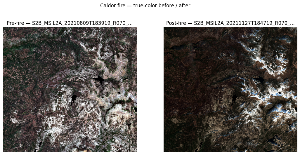
Walk through the three RS operator modules end-to-end on a real burn-scar scenario: the 2021 Caldor fire in El Dorado County, California, just south-west of Lake Tahoe. We compose:

gz.radiometry — ToFloat32 → DNToReflectance → PercentileClip → Gamma for a display pipeline; the same DNToReflectance powers the index chain.
gz.cloud — MaskFromSCL + gz.mask.ApplyMask to drop clouds and invalid pixels.
gz.indices — NBR (burn-sensitive), NDVI (vegetation), NDWI (water) computed from the same reflectance carrier via gz.Fanout. The burn signature lives in dNBR = NBR_pre − NBR_post.

Scenario.


AOI bbox (EPSG:4326)	`(-120.30, 38.55, -119.95, 38.95)` (Caldor fire core)
Pre-fire scene	`S2B_..20210809T..` (5 days before ignition, 0.1 % cloud)
Post-fire scene	`S2A_..20211112T..` (3 weeks after containment, 1.4 % cloud)
MGRS tile	`10SGH`
Bands	B02, B03, B04, B08, B12, SCL (BGRN + SWIR + scene-classification)

Caldor burned ~221,835 acres between 14 August and 21 October 2021, the second wildfire ever to cross the Sierra Nevada crest.

import geotoolz as gz
import matplotlib.pyplot as plt
import numpy as np
import planetary_computer
import pystac_client
import rioxarray
from georeader.geotensor import GeoTensor
from geotoolz.cloud import SCL_CLOUDS_AND_INVALID
from matplotlib.colors import ListedColormap
from rasterio.enums import Resampling

1. Load pre- and post-fire Sentinel-2 scenes¶

Search MPC for one cloud-free scene before ignition and one after containment, both on MGRS tile 10SGH. Load the spectral bands + SCL, resample everything to the 10 m grid.

BBOX = (-120.30, 38.55, -119.95, 38.95)
TARGET_TILE = "10SGH"

catalog = pystac_client.Client.open(
    "https://planetarycomputer.microsoft.com/api/stac/v1",
    modifier=planetary_computer.sign_inplace,
)


def _best_scene(date_range: str):
    items = list(
        catalog.search(
            collections=["sentinel-2-l2a"],
            bbox=BBOX,
            datetime=date_range,
            query={
                "eo:cloud_cover": {"lt": 5},
                "s2:mgrs_tile": {"eq": TARGET_TILE},
            },
        ).items()
    )
    return sorted(items, key=lambda x: x.properties["eo:cloud_cover"])[0]


pre = _best_scene("2021-07-01/2021-08-13")  # before ignition (Aug 14)
post = _best_scene("2021-10-22/2021-11-30")  # after containment (Oct 21)

print(f"pre  → {pre.id}  cloud={pre.properties['eo:cloud_cover']:.2f}%")
print(f"post → {post.id}  cloud={post.properties['eo:cloud_cover']:.2f}%")

pre  → S2B_MSIL2A_20210809T183919_R070_T10SGH_20210810T105317  cloud=0.07%
post → S2B_MSIL2A_20211127T184719_R070_T10SGH_20211128T194120  cloud=0.93%

def _load_band(item, key, *, ref=None, resampling=Resampling.bilinear):
    da = rioxarray.open_rasterio(item.assets[key].href, masked=False)
    da = da.squeeze("band", drop=True).rio.clip_box(*BBOX, crs="EPSG:4326")
    if ref is not None:
        da = da.rio.reproject_match(ref, resampling=resampling)
    return da


def _load_scene(item):
    """Load BGRN + SWIR + SCL aligned to the B04 (10 m) grid."""
    red = _load_band(item, "B04")
    green = _load_band(item, "B03", ref=red)
    blue = _load_band(item, "B02", ref=red)
    nir = _load_band(item, "B08", ref=red)
    swir = _load_band(item, "B12", ref=red)  # 20 m → 10 m bilinear
    scl = _load_band(item, "SCL", ref=red, resampling=Resampling.nearest)
    # Stack: B(0) G(1) R(2) NIR(3) SWIR(4)
    arr = np.stack(
        [blue.values, green.values, red.values, nir.values, swir.values],
        axis=0,
    ).astype("uint16")
    refl_gt = GeoTensor(
        values=arr,
        transform=red.rio.transform(),
        crs=red.rio.crs,
        fill_value_default=0,
    )
    scl_gt = GeoTensor(
        values=scl.values[None, ...].astype("uint8"),
        transform=scl.rio.transform(),
        crs=scl.rio.crs,
        fill_value_default=0,
    )
    return refl_gt, scl_gt


pre_refl, pre_scl = _load_scene(pre)
post_refl, post_scl = _load_scene(post)
print(f"pre_refl:  shape={pre_refl.shape}  dtype={pre_refl.dtype}")
print(f"post_refl: shape={post_refl.shape}  dtype={post_refl.dtype}")

pre_refl:  shape=(5, 2973, 3182)  dtype=uint16
post_refl: shape=(5, 2973, 3182)  dtype=uint16

2. Display pipeline — `ToFloat32 → DNToReflectance → PercentileClip → Gamma`¶

Build the standard four-stage gz.radiometry chain. ToFloat32 escapes the uint16 DN dtype, DNToReflectance applies the Sentinel-2 L2A scaling, PercentileClip is a robust per-band 2-98 % stretch, and Gamma brightens the midtones. All four are stock gz.radiometry operators — no custom code.

display_pipe = (
    gz.radiometry.ToFloat32()
    | gz.radiometry.DNToReflectance(scale=1e-4)
    | gz.radiometry.PercentileClip(p_min=2.0, p_max=98.0)
    | gz.radiometry.Gamma(g=1.2)
)
print(display_pipe)

pre_display = display_pipe(pre_refl)
post_display = display_pipe(post_refl)


def _rgb(stretched):
    """Pull R, G, B from the BGRN(+SWIR) stack and put channels last."""
    return np.transpose(np.asarray(stretched)[[2, 1, 0]], (1, 2, 0))


fig, ax = plt.subplots(1, 2, figsize=(13, 7))
ax[0].imshow(_rgb(pre_display))
ax[0].set_title(f"Pre-fire — {pre.id[:32]}…")
ax[0].axis("off")
ax[1].imshow(_rgb(post_display))
ax[1].set_title(f"Post-fire — {post.id[:32]}…")
ax[1].axis("off")
fig.suptitle("Caldor fire — true-color before / after", y=0.92)
plt.show()

Sequential([ToFloat32(), DNToReflectance(scale=0.0001, offset=0.0, axis=0), PercentileClip(p_min=2.0, p_max=98.0, axis=(-2, -1)), Gamma(g=1.2)])

3. Cloud masking — `MaskFromSCL`¶

gz.cloud.MaskFromSCL returns True where the SCL band’s value is in the supplied class set. Pair with gz.cloud.SCL_CLOUDS_AND_INVALID to drop clouds + cirrus + cloud shadows + no-data in one pass.

cloud_op = gz.cloud.MaskFromSCL(band_idx=0, classes=SCL_CLOUDS_AND_INVALID)
pre_mask = cloud_op(pre_scl)
post_mask = cloud_op(post_scl)
print(f"pre  mask: {float(np.mean(np.asarray(pre_mask))):.4f} fraction masked")
print(f"post mask: {float(np.mean(np.asarray(post_mask))):.4f} fraction masked")

pre  mask: 0.0007 fraction masked
post mask: 0.0302 fraction masked

4. Indices via `Fanout` — NDVI + NBR + NDWI from one reflectance carrier¶

gz.Fanout is sugar over a single-input Graph: one input, many named outputs. The Graph topologically sorts the nodes, so DNToReflectance runs exactly once and its output is shared by all three index ops — no redundant arithmetic.

NDVI ((NIR − Red)/(NIR + Red)) — vegetation
NBR ((NIR − SWIR)/(NIR + SWIR)) — burn severity (drops over scarred ground)
NDWI ((Green − NIR)/(Green + NIR)) — water / saturation

We also slot gz.mask.ApplyMask per scene to NaN out cloudy pixels.

def indices_pipe(cloud_mask):
    """Reflectance pipeline with cloud masking, computing 3 indices."""
    scale = gz.radiometry.DNToReflectance(scale=1e-4)
    drop_clouds = gz.mask.ApplyMask(mask=cloud_mask, fill_value=float("nan"))
    return scale | gz.Fanout(
        {
            "ndvi": gz.indices.NDVI(red_idx=2, nir_idx=3) | drop_clouds,
            "nbr": gz.indices.NBR(nir_idx=3, swir2_idx=4) | drop_clouds,
            "ndwi": gz.indices.NDWI(green_idx=1, nir_idx=3) | drop_clouds,
        }
    )


pre_idx = indices_pipe(pre_mask)(pre_refl)
post_idx = indices_pipe(post_mask)(post_refl)
print("pre keys :", list(pre_idx.keys()))
print("post keys:", list(post_idx.keys()))
for k in pre_idx:
    arr = np.asarray(pre_idx[k])
    lo, hi = float(np.nanmin(arr)), float(np.nanmax(arr))
    print(f"  pre  {k:5s}: range=[{lo: .3f}, {hi: .3f}]")

pre keys : ['ndvi', 'nbr', 'ndwi']
post keys: ['ndvi', 'nbr', 'ndwi']
  pre  ndvi : range=[-0.996,  0.999]
  pre  nbr  : range=[-0.999,  0.877]
  pre  ndwi : range=[-0.999,  0.997]

5. dNBR — the burn-severity signal¶

Subtract post-fire NBR from pre-fire NBR. Healthy unchanged vegetation cancels out; burned pixels show a strong positive differenced-NBR. USGS uses the threshold table:

dNBR	Severity
< 0.10	Unburned
0.10 – 0.27	Low
0.27 – 0.44	Moderate-low
0.44 – 0.66	Moderate-high
> 0.66	High

dnbr = np.asarray(pre_idx["nbr"]) - np.asarray(post_idx["nbr"])
print(
    f"dNBR range: [{np.nanmin(dnbr):.3f}, {np.nanmax(dnbr):.3f}]  "
    f"mean={np.nanmean(dnbr):.3f}"
)

# Severity classification map (USGS / FIRMS conventions).
bounds = np.array([-np.inf, 0.10, 0.27, 0.44, 0.66, np.inf])
labels = ["Unburned", "Low", "Mod-low", "Mod-high", "High"]
colors = ["#2c7bb6", "#abd9e9", "#ffffbf", "#fdae61", "#d7191c"]
class_map = np.digitize(dnbr, bounds[1:-1], right=False).astype(float)
class_map[np.isnan(dnbr)] = np.nan

dNBR range: [-1.949, 1.708]  mean=0.010

fig, ax = plt.subplots(1, 3, figsize=(18, 7))

ax[0].imshow(np.asarray(pre_idx["nbr"]), cmap="RdYlGn", vmin=-0.5, vmax=0.9)
ax[0].set_title("NBR — pre-fire")
ax[0].axis("off")

ax[1].imshow(np.asarray(post_idx["nbr"]), cmap="RdYlGn", vmin=-0.5, vmax=0.9)
ax[1].set_title("NBR — post-fire")
ax[1].axis("off")

cmap = ListedColormap(colors)
im = ax[2].imshow(class_map, cmap=cmap, vmin=-0.5, vmax=4.5)
ax[2].set_title("dNBR severity (USGS classes)")
ax[2].axis("off")
cbar = fig.colorbar(im, ax=ax[2], shrink=0.7, ticks=range(5))
cbar.ax.set_yticklabels(labels)

plt.show()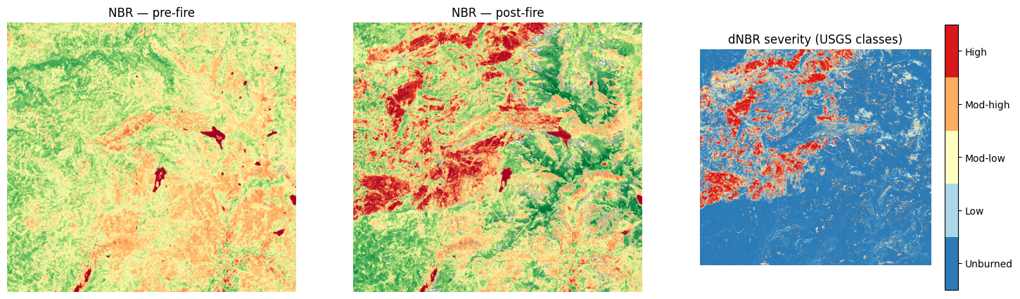

The right-hand panel is the burn footprint: cyan / blue pixels were unchanged forest, orange / red pixels are moderate-to-high burn severity — the Caldor scar.

6. NDVI loss — vegetation impact¶

The same Fanout shape lets us pull NDVI out of both scenes for free. Where vegetation burned, NDVI drops sharply; we visualise the raw post-fire NDVI alongside ΔNDVI.

delta_ndvi = np.asarray(post_idx["ndvi"]) - np.asarray(pre_idx["ndvi"])

fig, ax = plt.subplots(1, 2, figsize=(13, 7))
im0 = ax[0].imshow(np.asarray(post_idx["ndvi"]), cmap="RdYlGn", vmin=-0.4, vmax=0.9)
ax[0].set_title("NDVI — post-fire")
ax[0].axis("off")
fig.colorbar(im0, ax=ax[0], shrink=0.7, label="NDVI")

im1 = ax[1].imshow(delta_ndvi, cmap="RdBu", vmin=-0.6, vmax=0.6)
ax[1].set_title("ΔNDVI = post − pre")
ax[1].axis("off")
fig.colorbar(im1, ax=ax[1], shrink=0.7, label="ΔNDVI")

plt.show()

7. Summary¶

The three operator modules compose cleanly on real data:

gz.radiometry — ToFloat32 | DNToReflectance | PercentileClip | Gamma is the canonical display chain; DNToReflectance alone is the index-feed chain.
gz.cloud — MaskFromSCL(classes=SCL_CLOUDS_AND_INVALID) produces a True-where-bad mask in one line; pair with gz.mask.ApplyMask to drop those pixels as NaN.
gz.indices — every index (NDVI, NBR, NDWI, EVI, SAVI, MNDWI, …) has the same constructor shape (band indices, axis, epsilon), so they plug into Fanout interchangeably.

The composition primitives (|, Fanout) keep the multi-scene + multi-index logic linear and explicit: one reflectance carrier per scene, one Fanout per scene, then NumPy for the cross-scene diff. No custom operator subclasses required.

For the bigger picture — STAC discovery, tiled inference, multi-package composition — see the canonical multi-repo notebook: geocatalog/docs/notebooks/end_to_end_lake_tahoe.ipynb.