03 — Operators on Sentinel-2 (Lake Tahoe NDVI)

Composing a Sentinel-2 NDVI pipeline¶

This notebook is the operator-composition slice of the canonical Lake Tahoe scenario: cloud-free Sentinel-2 NDVI over Lake Tahoe, summer 2024. The end-to-end multi-repo flow (catalog discovery → patching → operators) lives in geocatalog/docs/notebooks/end_to_end_lake_tahoe.ipynb. Here we focus on the geotoolz part: composing named operators from gz.radiometry, gz.indices, gz.cloud, and gz.mask into linear and DAG-shaped pipelines.

Scenario.


AOI bbox (EPSG:4326)	`(-120.10, 38.92, -119.93, 39.27)` (Lake Tahoe main body)
Date range	`2024-06-01` to `2024-07-15` (peak-green Sierra window)
STAC	Microsoft Planetary Computer (`planetarycomputer.microsoft.com/api/stac/v1`)
Collection	`sentinel-2-l2a`
MGRS tile	`10SGJ` (fully covers the AOI; the other candidate `11SKD` only clips a sliver)
Cloud cover	< 5 %

The named operators we use:

Step	Operator	From
DN → reflectance	`DNToReflectance(scale=1e-4)`	`gz.radiometry`
Percentile stretch for the RGB preview	`PercentileClip(p_min=2, p_max=98)`	`gz.radiometry`
NDVI	`NDVI(red_idx=2, nir_idx=3)`	`gz.indices`
NDWI (water/vegetation complement)	`NDWI(green_idx=1, nir_idx=3)`	`gz.indices`
Cloud-class mask from SCL	`MaskFromSCL(classes=SCL_CLOUDS_AND_INVALID)`	`gz.cloud`
Drop masked pixels	`ApplyMask(mask=..., fill_value=np.nan)`	`gz.mask`

When you need to write a new operator that does not yet live in geotoolz, the Define an operator recipe walks through the contract.

1. Load one Sentinel-2 scene via Microsoft Planetary Computer¶

We use pystac-client to find one low-cloud scene in the AOI / date range, then rioxarray to load three bands: B04 (Red, 10 m), B08 (NIR, 10 m), and the SCL scene-classification band (20 m, resampled to the 10 m grid with nearest-neighbour). Red + NIR go into one carrier rn_gt (the reflectance pipeline input); SCL goes into a separate carrier scl_gt (the cloud-mask source).

import geotoolz as gz
import matplotlib.pyplot as plt
import numpy as np
import planetary_computer
import pystac_client
import rioxarray
import xarray as xr
from georeader.geotensor import GeoTensor
from geotoolz.cloud import SCL_CLOUDS_AND_INVALID
from rasterio.enums import Resampling

BBOX = (-120.10, 38.92, -119.93, 39.27)  # Lake Tahoe main body
# Peak-green window: post-snowmelt, pre-summer-drought. September Sierra
# scenes are technically cloud-free too but the vegetation is heat-
# stressed and NDVI plots wash out into orange.
DATE_RANGE = "2024-06-01/2024-07-15"
TARGET_TILE = "10SGJ"  # fully covers the AOI

catalog = pystac_client.Client.open(
    "https://planetarycomputer.microsoft.com/api/stac/v1",
    modifier=planetary_computer.sign_inplace,
)
search = catalog.search(
    collections=["sentinel-2-l2a"],
    bbox=BBOX,
    datetime=DATE_RANGE,
    query={
        "eo:cloud_cover": {"lt": 5},
        "s2:mgrs_tile": {"eq": TARGET_TILE},
    },
)
items = sorted(search.items(), key=lambda x: x.properties["eo:cloud_cover"])
print(f"found {len(items)} candidate items on tile {TARGET_TILE}")
item = items[0]
print(f"using {item.id}  cloud_cover={item.properties['eo:cloud_cover']:.1f}%")

found 17 candidate items on tile 10SGJ
using S2B_MSIL2A_20240614T183919_R070_T10SGJ_20240615T003207  cloud_cover=0.0%

def _load(
    asset_key: str,
    *,
    resample_to: xr.DataArray | None = None,
    resampling: Resampling = Resampling.bilinear,
) -> xr.DataArray:
    href = item.assets[asset_key].href
    da = rioxarray.open_rasterio(href, masked=False).squeeze("band", drop=True)
    da = da.rio.clip_box(*BBOX, crs="EPSG:4326")
    if resample_to is not None:
        da = da.rio.reproject_match(resample_to, resampling=resampling)
    return da


red = _load("B04")
green = _load("B03", resample_to=red)
blue = _load("B02", resample_to=red)
nir = _load("B08", resample_to=red)
scl = _load("SCL", resample_to=red, resampling=Resampling.nearest)

# Four-band reflectance carrier — B (idx 0), G (1), R (2), NIR (3) —
# uint16 DN values. Standard BGRN stacking; B04 → idx 2, B08 → idx 3.
bgrn_arr = np.stack([blue.values, green.values, red.values, nir.values], axis=0).astype(
    "uint16"
)
bgrn_gt = GeoTensor(
    values=bgrn_arr,
    transform=red.rio.transform(),
    crs=red.rio.crs,
    fill_value_default=0,
)

# Separate SCL carrier (1, H, W).
scl_gt = GeoTensor(
    values=scl.values[None, ...].astype("uint8"),
    transform=scl.rio.transform(),
    crs=scl.rio.crs,
    fill_value_default=0,
)

print(f"bgrn_gt: shape={bgrn_gt.shape}  dtype={bgrn_gt.dtype}")
print(f"scl_gt:  shape={scl_gt.shape}  dtype={scl_gt.dtype}")

bgrn_gt: shape=(4, 3935, 1599)  dtype=uint16
scl_gt:  shape=(1, 3935, 1599)  dtype=uint8

2. True-color reference¶

Before running the index, plot a percentile-stretched true-color composite so we know what the scene looks like. gz.radiometry.PercentileClip is the named op for the stretch; np.transpose reorders (C, H, W) → (H, W, C) for matplotlib.

rgb_pipe = gz.radiometry.DNToReflectance(scale=1e-4) | gz.radiometry.PercentileClip(
    p_min=2.0, p_max=98.0
)
rgb_full = rgb_pipe(bgrn_gt)
rgb_arr = np.asarray(rgb_full)[[2, 1, 0]]  # R, G, B from B-G-R-NIR

fig, ax = plt.subplots(figsize=(7, 8))
ax.imshow(np.transpose(rgb_arr, (1, 2, 0)))
ax.set_title(f"Lake Tahoe true-color (B04, B03, B02) — {item.id[:32]}…")
ax.axis("off")
plt.show()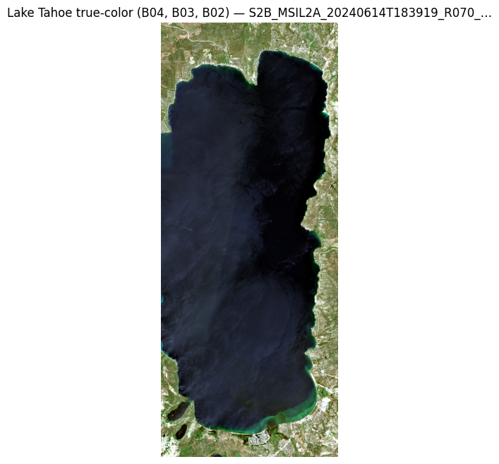

3. Compose NDVI with `Sequential`¶

The simplest possible shape — DN → reflectance, then NDVI. Two named ops, one |. BGRN stack → red is at idx 2, NIR at idx 3.

pipe = gz.radiometry.DNToReflectance(scale=1e-4) | gz.indices.NDVI(red_idx=2, nir_idx=3)
print(pipe)
ndvi_gt = pipe(bgrn_gt)
print("ndvi shape:", ndvi_gt.shape)
print(
    "ndvi range:",
    float(np.nanmin(np.asarray(ndvi_gt))),
    float(np.nanmax(np.asarray(ndvi_gt))),
)

Sequential([DNToReflectance(scale=0.0001, offset=0.0, axis=0), NDVI(nir_idx=3, red_idx=2, axis=0, eps=1e-10)])
ndvi shape: (3935, 1599)
ndvi range: -0.9999999992647058 0.999999999057493

4. Visualise the raw NDVI¶

Standard NDVI ramp. We use RdYlGn clipped at vmin=-0.4, vmax=0.9 so water shows red, conifer forest shows green, and the dry granite / scrub middle ground reads as a transition rather than alarming orange.

fig, ax = plt.subplots(figsize=(7, 8))
im = ax.imshow(np.asarray(ndvi_gt), cmap="RdYlGn", vmin=-0.4, vmax=0.9)
ax.set_title("NDVI (raw, no cloud mask)")
ax.axis("off")
fig.colorbar(im, ax=ax, shrink=0.7, label="NDVI")
plt.show()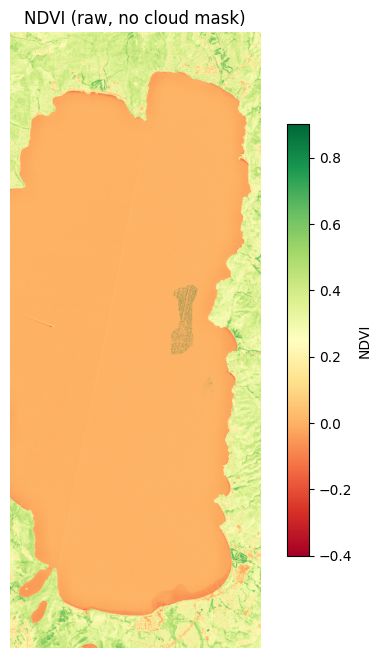

5. Cloud-aware variant¶

We extract a “drop these pixels” mask from SCL using gz.cloud.MaskFromSCL, then attach gz.mask.ApplyMask at the end of the same Sequential. The mask is True on cloud + invalid pixels; ApplyMask follows the library convention (“True = drop”) so the call is just ApplyMask(mask=cloud_mask, fill_value=np.nan).

cloud_op = gz.cloud.MaskFromSCL(
    band_idx=0,
    classes=SCL_CLOUDS_AND_INVALID,
)
cloud_mask = cloud_op(scl_gt)
print("cloud_mask shape:", cloud_mask.shape, "dtype:", cloud_mask.dtype)
print(f"fraction masked: {float(np.mean(np.asarray(cloud_mask))):.3f}")

clean_pipe = (
    gz.radiometry.DNToReflectance(scale=1e-4)
    | gz.indices.NDVI(red_idx=2, nir_idx=3)
    | gz.mask.ApplyMask(mask=cloud_mask, fill_value=float("nan"))
)
print(clean_pipe)
ndvi_clean = clean_pipe(bgrn_gt)
print(
    "clean ndvi range:",
    float(np.nanmin(np.asarray(ndvi_clean))),
    float(np.nanmax(np.asarray(ndvi_clean))),
)

cloud_mask shape: (3935, 1599) dtype: bool
fraction masked: 0.000
Sequential([DNToReflectance(scale=0.0001, offset=0.0, axis=0), NDVI(nir_idx=3, red_idx=2, axis=0, eps=1e-10), ApplyMask(mask={'type': 'ndarray', 'shape': [3935, 1599], 'dtype': 'bool'}, fill_value=nan, invert=False)])
clean ndvi range: -0.9999999992647058 0.999999999057493

fig, (ax1, ax2) = plt.subplots(1, 2, figsize=(13, 8))
ax1.imshow(np.transpose(rgb_arr, (1, 2, 0)))
ax1.set_title("True-color reference")
ax1.axis("off")
im2 = ax2.imshow(np.asarray(ndvi_clean), cmap="RdYlGn", vmin=-0.4, vmax=0.9)
ax2.set_title("Cloud-masked NDVI")
ax2.axis("off")
fig.colorbar(im2, ax=ax2, shrink=0.7, label="NDVI")
plt.show()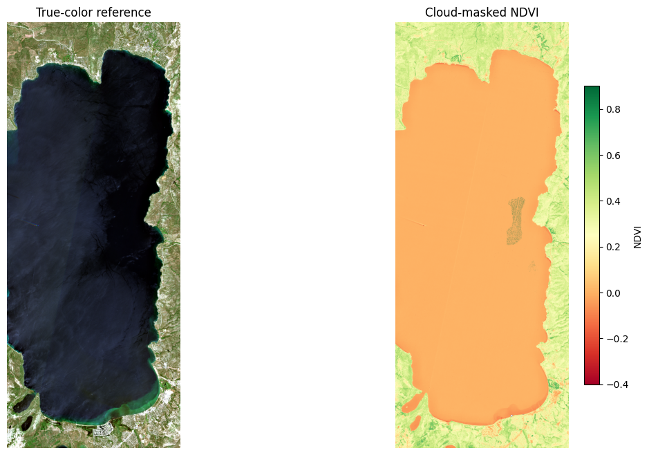

6. Fan-out — multiple indices from one scaled scene¶

gz.Fanout is sugar over a single-input Graph: one input, many named outputs. Here we compute NDVI and NDWI (the water-detection complement; high over open water, low over vegetation) off the same reflectance carrier — water and vegetation light up in opposite panels.

scaled = gz.radiometry.DNToReflectance(scale=1e-4)(bgrn_gt)
products = gz.Fanout(
    {
        "ndvi": gz.indices.NDVI(red_idx=2, nir_idx=3),
        "ndwi": gz.indices.NDWI(green_idx=1, nir_idx=3),
    }
)(scaled)
print("product keys:", list(products.keys()))
print("ndvi shape:", products["ndvi"].shape)
print("ndwi shape:", products["ndwi"].shape)

product keys: ['ndvi', 'ndwi']
ndvi shape: (3935, 1599)
ndwi shape: (3935, 1599)

fig, axes = plt.subplots(1, 2, figsize=(13, 8))
cfg = [("ndvi", "RdYlGn", (-0.4, 0.9)), ("ndwi", "Blues", (-0.4, 0.6))]
for ax, (name, cmap, (vmin, vmax)) in zip(axes, cfg, strict=True):
    im = ax.imshow(np.asarray(products[name]), cmap=cmap, vmin=vmin, vmax=vmax)
    ax.set_title(name.upper())
    ax.axis("off")
    fig.colorbar(im, ax=ax, shrink=0.7, label=name)
plt.show()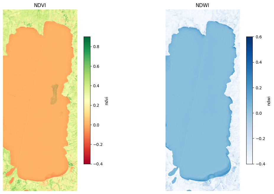

7. Observability — inspect, time, assert¶

Operator is general enough that side-effects round-trip the same as transforms. pipekit ships a small library of identity-with-side- effect ops you compose inline:

Primitive	Role	Re-exported as
`Tap(fn, name=...)`	callback hook (logging / breakpoints)	`gz.Tap`
`ShapeTrace(mode="diff_only")`	log `shape`/`dtype` on change	`gz.ShapeTrace`
`Snapshot()` + `snap.at(key)`	capture intermediates by key	`gz.Snapshot`
`Profile()` + `prof.wrap(op)`	per-step wall-clock	`from pipekit import Profile`
`AssertShape(expected)`	runtime contract; raises `QCError`	`from pipekit import AssertShape`
`AssertDType(expected)`	runtime dtype contract	`from pipekit import AssertDType`
`Quarantine(check, sentinel)`	non-raising QC (route bad inputs)	`from pipekit import Quarantine`

None of these change the pipeline output — they just observe or enforce. Drop them in with |, take them out for production.

from pipekit import AssertDType, AssertShape, Profile


snap = gz.Snapshot()
prof = Profile()

# Same NDVI pipeline as §3, but instrumented:
#   - AssertShape pins the input contract (4 bands, any H × W)
#   - Tap logs the dtype on the first call
#   - Snapshot.at captures the reflectance intermediate by key
#   - ShapeTrace prints when shape/dtype changes between steps
#   - Profile.wrap times each operator
#   - AssertDType pins the output contract
trace = gz.ShapeTrace(mode="diff_only", label="ndvi")

observed = (
    AssertShape((4, None, None))
    | gz.Tap(lambda gt: print(f"input dtype: {np.asarray(gt).dtype}"), name="log_dtype")
    | prof.wrap(gz.radiometry.DNToReflectance(scale=1e-4))
    | snap.at("reflectance")
    | trace
    | prof.wrap(gz.indices.NDVI(red_idx=2, nir_idx=3))
    | trace
    | AssertDType("float64")
)
_ = observed(bgrn_gt)

print("\nSnapshot keys:", list(snap.captures))
print(
    "reflectance carrier:",
    snap.captures["reflectance"].shape,
    snap.captures["reflectance"].dtype,
)
print("\nProfile report:")
for name, stats in prof.report().items():
    print(
        f"  {name:20s}  calls={int(stats['calls'])}  mean={stats['mean'] * 1000:6.1f} ms"
    )

input dtype: uint16
[ndvi] shape=(4, 3935, 1599) dtype=float64
[ndvi] shape=(3935, 1599) dtype=float64

Snapshot keys: ['reflectance']
reflectance carrier: (4, 3935, 1599) float64

Profile report:
  DNToReflectance       calls=1  mean=  32.9 ms
  NDVI                  calls=1  mean=  17.2 ms

What you’d reach for next:

Quarantine — route bad-cloud-fraction scenes to a sentinel instead of aborting the batch.
Cache — memoize by config + input hash for expensive ops (Ledoit-Wolf covariance, learned models).
Try / Coalesce / Retry — production control flow for flaky external loaders (STAC, S3).

Each is itself an Operator so the whole stack composes uniformly.

8. When to use which composition primitive¶

The cells above used Sequential (linear) and Fanout (one input, many outputs). The choice tree for the rest:

You want…	Reach for	Why
A linear chain of 2–6 ops	`Sequential` (or `op_a \| op_b`)	Smallest API surface; flattens nested pipes.
Named intermediates / branching / fan-in	`Graph`	Same scene, multiple sub-pipelines, fused at the end.
Runtime two-way fork (e.g. reproject if geographic)	`Branch`	Predicate evaluates the whole carrier.
Sensor / product dispatch (`'S2'` vs `'L8'`)	`Switch`	Finite named cases; default is `Identity`.
One input → many named derived products	`Fanout`	Sugar over a single-input `Graph`.

Each of these is itself an Operator, so they nest freely: a Graph inside a Sequential, a Switch whose cases are Sequentials, a Fanout whose values are Graphs.

8. Where next¶

End-to-end Lake Tahoe (cross-repo): the canonical multi-package walkthrough lives in geocatalog/docs/notebooks/end_to_end_lake_tahoe.ipynb — STAC discovery → catalog loading → patching → operators.
Define your own operator: when something is not in the named-op surface yet, write a subclass — see Define an operator.
More composition patterns: the pipeline idioms notebook is a recipe gallery of observer / control-flow / QC patterns.
Deployment shapes: the deployment shapes notebook tours 13 deployment patterns (notebook, ETL, FastAPI, tile server, …).
Concepts: the Concepts page explains the model behind these primitives with diagrams.
Recipes: Branching pipelines, Integration with geocatalog & geopatcher.