06 — ML patches + augmentations

ML patches — augmentations + tiled inference¶

The companion to Patching: grid → process → stitch. Same patcher / Field / gz.patch_ops machinery, but now the per-chip work is the ML inference path: load → augment (training-time only) → model → stitch into a per-pixel classification map.

We demonstrate three slices of the package on a real Sentinel-2 scene:

Stage	Module	Ops
Training-chip extraction (irregular sampling)	`geopatcher`	`SpatialJitteredStride`
Per-chip augmentation	`gz.augment`	`Compose([RandomFlip, RandomRotate90, BrightnessJitter, GaussianNoise])`
Inference + carrier wrap	`gz.ModelOp`	`ModelOp(model, method="predict")`
Vote-stitching of classification labels	`geopatcher`	`SpatialHardVote(n_classes=3)`

The “model” is a rule-based three-class classifier driven by NDVI + NDWI thresholds — water (0), bare/scrub (1), vegetation (2). It plays the role of any real sklearn / PyTorch estimator: anything with a predict method (or __call__) plugs into ModelOp interchangeably.

import geopatcher as gp
import geotoolz as gz
import matplotlib.pyplot as plt
import numpy as np
import planetary_computer
import pystac_client
import rioxarray
from geopatcher.fields import RasterField
from georeader.geotensor import GeoTensor
from geotoolz.patch_ops import ApplyToChips, GridSampler, Stitch
from matplotlib.colors import ListedColormap
from rasterio.enums import Resampling

1. Load one Sentinel-2 scene¶

Lake Tahoe, same scene as the companion patching notebook. BGRN (4 bands) — we want green + NIR for NDWI and red + NIR for NDVI.

BBOX = (-120.10, 38.92, -119.93, 39.27)

catalog = pystac_client.Client.open(
    "https://planetarycomputer.microsoft.com/api/stac/v1",
    modifier=planetary_computer.sign_inplace,
)
items = sorted(
    catalog.search(
        collections=["sentinel-2-l2a"],
        bbox=BBOX,
        datetime="2024-06-01/2024-07-15",
        query={
            "eo:cloud_cover": {"lt": 5},
            "s2:mgrs_tile": {"eq": "10SGJ"},
        },
    ).items(),
    key=lambda x: x.properties["eo:cloud_cover"],
)
item = items[0]
print(f"using {item.id}")

using S2B_MSIL2A_20240614T183919_R070_T10SGJ_20240615T003207

def _load(key, *, ref=None, resampling=Resampling.bilinear):
    da = rioxarray.open_rasterio(item.assets[key].href, masked=False)
    da = da.squeeze("band", drop=True).rio.clip_box(*BBOX, crs="EPSG:4326")
    if ref is not None:
        da = da.rio.reproject_match(ref, resampling=resampling)
    return da


red = _load("B04")
green = _load("B03", ref=red)
blue = _load("B02", ref=red)
nir = _load("B08", ref=red)

# Reflectance up front so augmentations and the model see physical units.
dn_stack = np.stack([blue.values, green.values, red.values, nir.values], axis=0).astype(
    "uint16"
)
refl = gz.radiometry.DNToReflectance(scale=1e-4)(
    GeoTensor(
        values=dn_stack,
        transform=red.rio.transform(),
        crs=red.rio.crs,
        fill_value_default=0,
    )
)
print(f"reflectance carrier: shape={refl.shape}  dtype={refl.dtype}")

reflectance carrier: shape=(4, 3935, 1599)  dtype=float64

2. Training-chip sampling — `SpatialJitteredStride`¶

For a training dataset we don’t want a regular grid (every chip lines up the same way and overfits to position); we want jittered anchors so the model sees translated variants of similar terrain. SpatialJitteredStride(step, jitter) perturbs each regular-grid anchor by a uniform random offset bounded by jitter pixels.

Compare to SpatialPoissonDisk — Poisson-disk sampling places anchors as far apart as possible (minimum-distance constraint), giving the most spatially-diverse training chips. Use it when training samples are expensive (annotated labels) and you want maximum coverage per chip.

field = RasterField(reader=refl)
train_patcher = gp.SpatialPatcher(
    geometry=gp.SpatialRectangular(size=(128, 128)),
    # jitter is in step-units (0.0 = none, 0.5 = ± half a step), so
    # 0.25 of a 192-px step gives ±48 px of jitter per anchor.
    sampler=gp.SpatialJitteredStride(step=(192, 192), jitter=0.25, seed=0),
    window=gp.SpatialBoxcar(),
    aggregation=gp.SpatialOverlapAdd(),
)
train_chips = list(train_patcher.split(field))
print(f"sampled {len(train_chips)} training chips of size 128×128")

sampled 160 training chips of size 128×128

def _rgb(arr):
    """(C, H, W) reflectance → (H, W, 3) display range."""
    rgb = np.transpose(arr[[2, 1, 0]], (1, 2, 0))  # R, G, B
    lo, hi = np.nanpercentile(rgb, [2, 98])
    return np.clip((rgb - lo) / (hi - lo + 1e-9), 0, 1)


fig, axes = plt.subplots(2, 4, figsize=(14, 7))
for ax, chip in zip(axes.flat, train_chips[:8], strict=False):
    ax.imshow(_rgb(np.asarray(chip.data)))
    ax.set_title(
        f"chip @ row={chip.indices.row_off}\n col={chip.indices.col_off}",
        fontsize=9,
    )
    ax.axis("off")
fig.suptitle("8 jittered training chips (128 × 128, ±48 px jitter)", y=1.0)
plt.tight_layout()
plt.show()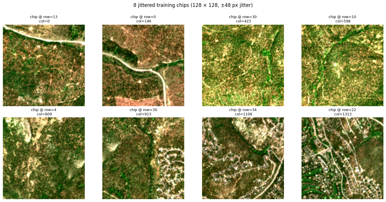

3. Augment one chip with `gz.augment.Compose`¶

A typical RS-safe augmentation pipeline: random flips, 90° rotations, brightness jitter (multiplicative gain), and Gaussian sensor noise. Each gz.augment.* op:

preserves CRS and updates the affine transform (so flips and rotations still map to the right world coordinates),
is reproducible — pass seed=... for a deterministic draw or omit for entropy from the OS,
composes via gz.augment.Compose(ops, p=...) so the whole chain has a single overall-probability gate.

augment = gz.augment.Compose(
    [
        gz.augment.RandomFlip(p_horizontal=0.5, p_vertical=0.5),
        gz.augment.RandomRotate90(p=0.75),
        gz.augment.BrightnessJitter(factor=(0.85, 1.15), per_band=True),
        gz.augment.GaussianNoise(sigma=0.01),
    ],
    p=1.0,
)
print(augment)

base = train_chips[0].data
fig, axes = plt.subplots(1, 5, figsize=(17, 4))
axes[0].imshow(_rgb(np.asarray(base)))
axes[0].set_title("original")
axes[0].axis("off")
for ax, seed in zip(axes[1:], range(4), strict=True):
    aug = augment(base, seed=seed)
    ax.imshow(_rgb(np.asarray(aug)))
    ax.set_title(f"augmented (seed={seed})")
    ax.axis("off")
fig.suptitle("Same chip, 4 augmented draws", y=1.02)
plt.tight_layout()
plt.show()

Compose(augmentations=[{'class': 'RandomFlip', 'config': {'p_horizontal': 0.5, 'p_vertical': 0.5, 'seed': None}}, {'class': 'RandomRotate90', 'config': {'p': 0.75, 'seed': None}}, {'class': 'BrightnessJitter', 'config': {'factor': (0.85, 1.15), 'per_band': True, 'seed': None}}, {'class': 'GaussianNoise', 'config': {'sigma': 0.01, 'per_band': True, 'seed': None}}], p=1.0, seed=None)

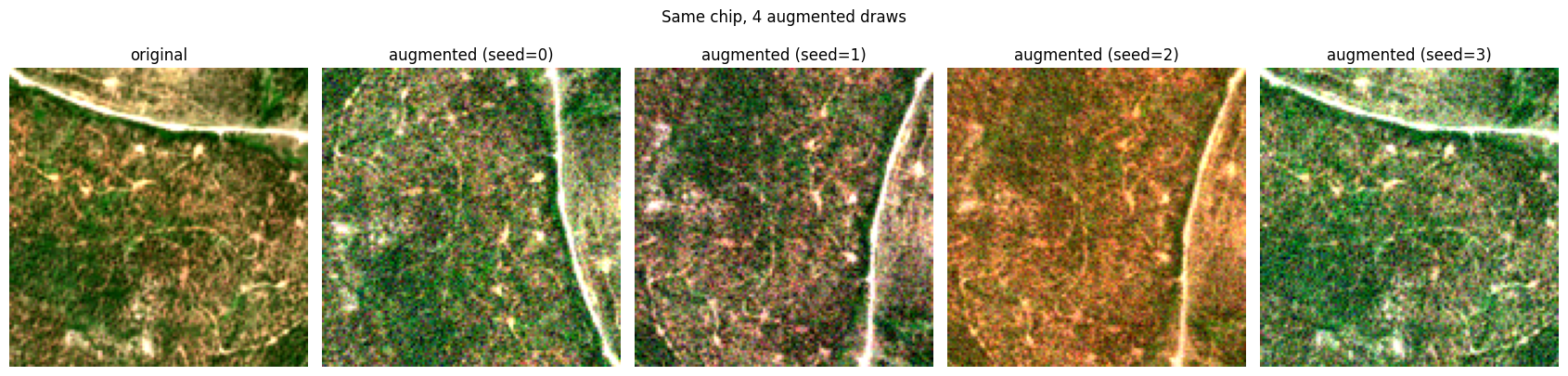
Notice each draw is different (flips, rotations, brightness shifts all sample independently per seed) but always preserves the CRS + spatial extent semantics. That’s the reproducible-RS-augmentation contract gz.augment enforces.

4. A three-class rule-based “model”¶

To keep this notebook self-contained we use a small NDVI / NDWI threshold rule as our classifier. Any callable with a predict method (sklearn) or __call__ (PyTorch / JAX) drops in via gz.ModelOp the same way — ModelOp is the substrate adapter.

Classes:

id	name	rule
0	Water	`NDWI > 0.1`
1	Bare / scrub	`NDVI < 0.25` and not water
2	Vegetation	`NDVI ≥ 0.25`

class NDVIClassifier:
    """Rule-based 3-class classifier with the sklearn-style `predict` API."""

    def predict(self, x: np.ndarray) -> np.ndarray:
        # x is (4, H, W) reflectance — B(0) G(1) R(2) NIR(3).
        green, red, nir_ = x[1], x[2], x[3]
        ndvi = (nir_ - red) / (nir_ + red + 1e-10)
        ndwi = (green - nir_) / (green + nir_ + 1e-10)
        labels = np.full(ndvi.shape, 1, dtype=np.int64)  # default: bare/scrub
        labels[ndwi > 0.1] = 0  # water
        labels[ndvi >= 0.25] = 2  # vegetation
        return labels


model_op = gz.ModelOp(NDVIClassifier(), method="predict")
print(model_op)

# Smoke-test on a single chip.
sample_out = model_op(base)
print(f"single-chip output: shape={sample_out.shape}  dtype={sample_out.dtype}")
print(f"class counts:      {np.bincount(np.asarray(sample_out).ravel(), minlength=3)}")

ModelOp(model_type='NDVIClassifier', method='predict', batch_size=None)
single-chip output: shape=(128, 128)  dtype=int64
class counts:      [    0   926 15458]

5. Tiled inference — `Sequential([GridSampler, ApplyToChips, Stitch])`¶

Now the full pipeline. The per-chip op is ModelOp(...) instead of the NDVI from the previous notebook; the aggregation is SpatialHardVote(n_classes=3) instead of SpatialOverlapAdd because we are stitching integer class labels, not continuous values.

For inference we also use a denser, non-jittered sampler (SpatialRegularStride) — jitter is a training-time trick, not an inference-time one.

infer_patcher = gp.SpatialPatcher(
    geometry=gp.SpatialRectangular(size=(256, 256)),
    sampler=gp.SpatialRegularStride(step=(256, 256)),
    window=gp.SpatialBoxcar(),
    aggregation=gp.SpatialHardVote(n_classes=3),
)
inference = gz.Sequential(
    [
        GridSampler(patcher=infer_patcher),
        ApplyToChips(operator=model_op),
        Stitch(aggregation=infer_patcher.aggregation, domain=field.domain),
    ]
)
print(inference)

class_map = np.asarray(inference(field))
# Domain has channel axis (4, H, W); SpatialHardVote produces (4, H, W)
# with each channel a duplicate of the (H, W) vote map. Collapse:
if class_map.ndim == 3:
    class_map = class_map[0]
print(f"classification map: shape={class_map.shape}  dtype={class_map.dtype}")
print(f"class counts:      {np.bincount(class_map.ravel(), minlength=3)}")

Sequential([GridSampler(patcher={'geometry': {'class': 'SpatialRectangular', 'config': {'size': [256, 256]}}, 'sampler': {'class': 'SpatialRegularStride', 'config': {'step': [256, 256]}}, 'window': {'class': 'SpatialBoxcar', 'config': {}}, 'aggregation': {'class': 'SpatialHardVote', 'config': {'n_classes': 3}}}), ApplyToChips(operator={'class': 'ModelOp', 'config': {'model_type': 'NDVIClassifier', 'method': 'predict', 'batch_size': None}}), Stitch(aggregation={'class': 'SpatialHardVote', 'config': {'n_classes': 3}})])

classification map: shape=(3935, 1599)  dtype=int64
class counts:      [ 546953 4559300 1185812]

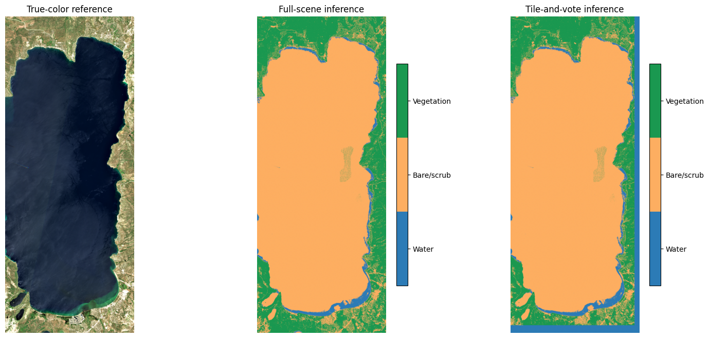
6. Compare against full-scene inference¶

Run the same model on the whole scene without patching as a reference. The patched output should match across the interior.

full_class_map = np.asarray(model_op(refl))
agree = float(np.mean(class_map == full_class_map))
print(f"per-pixel agreement: {agree * 100:.2f}%")

fig, axes = plt.subplots(1, 3, figsize=(18, 8))

labels = ["Water", "Bare/scrub", "Vegetation"]
class_cmap = ListedColormap(["#2c7bb6", "#fdae61", "#1a9850"])

axes[0].imshow(_rgb(np.asarray(refl)))
axes[0].set_title("True-color reference")
axes[0].axis("off")

im1 = axes[1].imshow(full_class_map, cmap=class_cmap, vmin=-0.5, vmax=2.5)
axes[1].set_title("Full-scene inference")
axes[1].axis("off")
cbar = fig.colorbar(im1, ax=axes[1], shrink=0.7, ticks=range(3))
cbar.ax.set_yticklabels(labels)

im2 = axes[2].imshow(class_map, cmap=class_cmap, vmin=-0.5, vmax=2.5)
axes[2].set_title("Tile-and-vote inference")
axes[2].axis("off")
cbar = fig.colorbar(im2, ax=axes[2], shrink=0.7, ticks=range(3))
cbar.ax.set_yticklabels(labels)
plt.show()

per-pixel agreement: 93.76%

7. Recap¶

The same three-op patching pattern from 05 — Patching: grid → process → stitch hosts the ML inference path with zero structural change — only the parts that need to vary do:

What	Patching demo	ML demo
Sampler	`SpatialRegularStride` (every pixel covered)	`SpatialJitteredStride` (training) or `SpatialRegularStride` (inference)
Window	`SpatialHann` (smooth blending)	`SpatialBoxcar` (votes don’t need blending)
Per-chip op	NDVI	`gz.ModelOp(model, method="predict")`
Aggregation	`SpatialOverlapAdd` (continuous map)	`SpatialHardVote(n_classes=K)` (class labels)

Other building blocks worth pairing in:

gz.augment — Compose([RandomFlip, RandomRotate90, BrightnessJitter, GaussianNoise, AtmosphericHaze, SimulatedClouds, CutMix, ...]) for training-chip augmentation. Each op preserves CRS / transform so the augmented carrier is still geographically valid.
SklearnOp — gz.learn.SklearnOp(estimator, mode="pixel") if you want a fitted sklearn estimator (RandomForestClassifier, GBM, kNN, …) instead of a hand-coded rule.
SpatialSoftVote — like HardVote but stitches per-class probabilities (chip outputs shape (K, H, W)), letting you threshold or compute class margins at the field level.
Profile + ShapeTrace from the observability section of operators_lake_tahoe — wrap ModelOp to time per-chip inference cost across the run.

For the cross-package walk-through (STAC → catalog → patcher → operators), see geocatalog/docs/notebooks/end_to_end_lake_tahoe.ipynb.