Non-stationary GEV — a state-space GP trend

Abstract¶

The line committed to a shape; the ODE committed to a mechanism. The final model lets the data shape the trend — but with a smoothness prior tuned to resist over-fitting a single short record. We write the GEV location as $\mu(t)=\mu_0+f(t)$ with $f$ a Gaussian process in state-space form, and choose the local linear trend (an integrated random walk): the trend’s slope random-walks, so draws default to a straight line and bend only where the data insist. It is a stochastic differential equation — the noise-driven sibling of the previous notebook’s ODE — walked as a Markov chain in $O(n)$ . We fit it with NUTS, show why a free stationary GP over-fits where this one does not, put line, ODE, and GP on one set of axes, and close the series.

Keywords:non-stationary extremesGEVGaussian processstate space modellocal linear trendNUTS¶

Non-stationary extremes: a state-space Gaussian process¶

Three notebooks, three answers to one question — how does the GEV location move through time?

Non-stationary GEV — a parametric trend: a line. Strong, interpretable, rigid.
Non-stationary GEV — a mechanistic ODE: an ODE. A forced relaxation with physical memory τ — it can bend, but only in the one shape its mechanism allows.
this notebook: a Gaussian process. A smoothness prior that lets the data shape the trend, while defaulting to a straight line where they are silent.

The GP is the natural endpoint, but two cautions shape the design. A textbook GP over $n$ times needs an $n\times n$ covariance and $O(n^3)$ work — so we use the state-space form, which is also conceptually perfect here: it turns the GP into a stochastic differential equation, the direct generalisation of the ODE we just fitted. And a stationary GP with a free lengthscale will happily chase multidecadal wiggles and over-fit ~115 maxima — so we choose a trend prior built to stay smooth.

Background¶

A GP prior on the trend¶

We model the location as a draw from a Gaussian process,

\mu(t) = \mu_0 + f(t), \qquad f \sim \mathcal{GP}\!\bigl(0,\; k(t,t')\bigr).

((1))

The choice of covariance is the whole story. A stationary Matérn kernel with a free lengthscale $\ell$ is flexible in both directions: give it a short $\ell$ and it will track every multidecadal excursion in a century of annual maxima, fitting noise as if it were trend. On a single short record that is over-fitting — we demonstrate it below.

The local linear trend¶

Instead we use the local linear trend, the smooth-trend prior at the heart of structural time-series models. The idea: the trend has a level and a slope, the level moves at the current slope, and only the slope is nudged by noise:

\frac{\mathrm d}{\mathrm dt}\begin{pmatrix} f \\ f' \end{pmatrix} = \begin{pmatrix}0&1\\0&0\end{pmatrix}\begin{pmatrix} f \\ f' \end{pmatrix} + \begin{pmatrix}0\\1\end{pmatrix}\,\sigma_s\,\mathrm{d}\beta(t).

((2))

This is an integrated random walk (the level integrates a random-walking slope), and it is exactly a Gaussian process — with a non-stationary kernel whose draws are smooth, near-linear curves. The single knob $\sigma_s$ (the slope-diffusion) sets how far the trend may bend: as $\sigma_s\to 0$ it is a straight line; the larger it is, the more curvature the data can buy. “Linear unless the data insist.”

Compare the previous notebook’s energy balance, $\tau\,\dot T=\beta F(t)-T$ : that was a deterministic relaxation toward a known forcing; ((2)) is a stochastic drift whose direction itself diffuses. Same state-space lineage — the forcing is replaced by randomness.

From SDE to a Markov chain¶

Sampled at the observation years, ((2)) is a linear-Gaussian recursion — a Markov chain — with closed-form, $\ell$ -free matrices:

\mathbf{x}_k = \underbrace{\begin{pmatrix}1&\Delta_k\\0&1\end{pmatrix}}_{\mathbf A_k}\mathbf{x}_{k-1} + \mathbf{q}_k, \qquad \mathbf Q_k = \sigma_s^2\begin{pmatrix}\Delta_k^3/3 & \Delta_k^2/2\\ \Delta_k^2/2 & \Delta_k\end{pmatrix}.

((3))

We walk it with non-centered innovations — $O(n)$ work, no big matrix — and let NUTS infer the initial slope, $\sigma_s$ , $\mu_0$ , and the GEV parameters jointly with the path.

Setup¶

import sys
import pathlib

try:
    import spatial_extremes  # noqa: F401  installed editable in the project venv
except ModuleNotFoundError:
    _here = pathlib.Path.cwd().resolve()
    _roots = (_here, *_here.parents)
    _cands = [r / "src" for r in _roots]
    _cands += [r / "projects" / "spatial_extremes" / "src" for r in _roots]
    _src = next((c for c in _cands if (c / "spatial_extremes").exists()), None)
    if _src is None:
        raise RuntimeError("cannot locate spatial_extremes/src") from None
    sys.path.insert(0, str(_src))

from __future__ import annotations

import warnings
warnings.filterwarnings("ignore", message=r".*IProgress.*")

import jax
jax.config.update("jax_enable_x64", True)

import numpy as np
import pandas as pd
import jax.numpy as jnp
import jax.random as jr
from jax.lax import scan
from jax.scipy.special import logsumexp
import matplotlib.pyplot as plt
import seaborn as sns

import numpyro
import numpyro.distributions as ndist
from numpyro.infer import MCMC, NUTS
from numpyro.infer.initialization import init_to_median

from diffrax import ODETerm, Tsit5, diffeqsolve, SaveAt, ConstantStepSize

from xtremax import GeneralizedExtremeValueDistribution as GEV
from xtremax import gev_log_prob, gev_survival

from spatial_extremes import data

sns.set_theme(style="whitegrid", context="notebook", palette="deep")

# Same long station: Albacete, 1901-2025.
years, maxima, meta = data.load_single_station()
place = meta["name"]
y_np = np.asarray(maxima, float)
yr = np.asarray(years, int)
n = y_np.size
y = jnp.asarray(y_np)
y_mean, y_std = float(y.mean()), float(y.std())
dts = jnp.asarray(np.diff(yr).astype(float))   # (n-1,) year gaps between maxima
eye = jnp.eye(2)

print("source:", "REAL CDS" if meta["is_real"] else "synthetic")
print(f"{place} — id {meta['station_id']}, {n} annual maxima, {yr.min()}-{yr.max()}")

source: REAL CDS
Albacete — id SP000008280, 115 annual maxima, 1901-2025

The state-space trend¶

llt_trend(slope0, sigma_s, z) walks the Markov chain ((3)): starting from level 0 and an initial slope, it applies the closed-form transition $\mathbf A_k$ and process noise $\mathbf Q_k$ for each year gap, propagating non-centered innovations z through a jax.lax.scan. It returns the trend value $f_k$ at every year — the whole GP in one linear pass, no lengthscale required.

def llt_trend(slope0, sigma_s, z):
    # Local linear trend (integrated random walk). State x = [level, slope].
    # level integrates the slope; only the slope is driven by noise. Non-centered.
    x0 = jnp.array([0.0, slope0])                      # mu0 carries the offset

    def step(x_prev, inp):
        dt, zk = inp
        A = jnp.array([[1.0, dt], [0.0, 1.0]])         # A_k = exp(F dt)
        Q = sigma_s**2 * jnp.array([[dt**3 / 3, dt**2 / 2],
                                    [dt**2 / 2, dt]])   # integrated-Wiener noise
        x = A @ x_prev + jnp.linalg.cholesky(Q + 1e-12 * eye) @ zk
        return x, x[0]

    _, fs = scan(step, x0, (dts, z))
    return jnp.concatenate([x0[:1], fs])               # (n,) trend f_k

Draw from the prior at three slope-diffusions. At $\sigma_s=0$ the trend is a straight line set by its initial slope; as $\sigma_s$ grows the line is allowed to bend, but it never wiggles like a stationary kernel — the prior belief is “smooth, and linear unless pushed”. This is the regularisation that keeps a century of maxima from being over-fit.

fig, axes = plt.subplots(1, 3, figsize=(13, 3.6), sharey=True)
for ax, sig in zip(axes, (0.0, 0.003, 0.012)):
    for s in range(6):
        key = jr.PRNGKey(s)
        slope0 = 0.02 * jr.normal(key)
        zz = jr.normal(jr.fold_in(key, 1), (n - 1, 2))
        ax.plot(yr, y_mean + np.asarray(llt_trend(slope0, sig, zz)), lw=1.4, alpha=0.85)
    ax.set(xlabel="year", title=f"prior draws, sigma_s = {sig:g}")
axes[0].set_ylabel("mu(t) prior (degC)")
fig.tight_layout()
plt.show()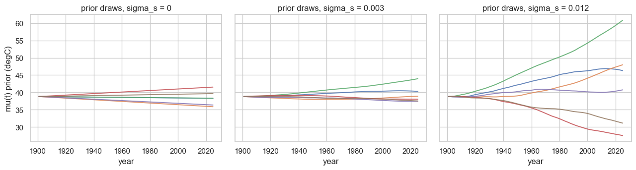

The model¶

The GEV likelihood with the local-linear-trend location. We sample the initial slope, the slope-diffusion $\sigma_s$ (a tight half-normal — the data may bend the line but must pay for it), the GEV scale/shape, and the $2(n{-}1)$ non-centered innovations. NUTS infers the joint posterior over hyperparameters and the path.

def gev_llt(obs):
    mu0 = numpyro.sample("mu0", ndist.Normal(y_mean, 5.0))
    slope0 = numpyro.sample("slope0", ndist.Normal(0.0, 0.05))        # degC/yr
    sigma_s = numpyro.sample("sigma_s", ndist.HalfNormal(0.003))      # slope diffusion
    log_sigma = numpyro.sample("log_sigma", ndist.Normal(np.log(y_std), 0.5))
    xi = numpyro.sample("xi", ndist.Normal(0.0, 0.25))
    z = numpyro.sample("z", ndist.Normal(0, 1).expand([n - 1, 2]).to_event(2))
    f = llt_trend(slope0, sigma_s, z)
    numpyro.sample("obs", GEV(loc=mu0 + f, scale=jnp.exp(log_sigma),
                              concentration=xi), obs=obs)

mcmc = MCMC(NUTS(gev_llt, target_accept_prob=0.95, init_strategy=init_to_median),
            num_warmup=1000, num_samples=1000, num_chains=2,
            chain_method="vectorized", progress_bar=False)
mcmc.run(jr.PRNGKey(0), y)
post = mcmc.get_samples()
n_div = int(mcmc.get_extra_fields()["diverging"].sum())
for k in ("mu0", "slope0", "sigma_s", "xi"):
    s = np.asarray(post[k])
    print(f"{k:9s} median {np.median(s):9.4f}   90% ({np.quantile(s,.05):.4f}, "
          f"{np.quantile(s,.95):.4f})")
print(f"divergences: {n_div} / {post['xi'].size}")

mu0       median   38.0785   90% (37.2030, 39.0196)
slope0    median   -0.0174   90% (-0.0645, 0.0132)
sigma_s   median    0.0039   90% (0.0009, 0.0078)
xi        median   -0.1145   90% (-0.1876, -0.0207)
divergences: 9 / 2000

Reading the trend¶

$\sigma_s$ is the bend budget — how far the slope may wander from a constant. It comes out small, so the trend stays close to a line; the warming is summarised robustly as the difference between the trend’s first and last 15-year means.

def ci(a): return np.quantile(a, [0.025, 0.5, 0.975])
NS = 600
sub = jr.choice(jr.PRNGKey(1), post["xi"].size, (NS,), replace=False)
f_draws = jax.vmap(lambda s0, ss, zz: llt_trend(s0, ss, zz))(
    post["slope0"][sub], post["sigma_s"][sub], post["z"][sub])
mu_draws = np.asarray(post["mu0"][sub][:, None] + f_draws)      # (NS, n)
early = mu_draws[:, yr <= yr.min() + 15].mean(1)
late = mu_draws[:, yr >= yr.max() - 15].mean(1)
realized = late - early
rlo, rmd, rhi = ci(realized)
print(f"warming (last 15yr - first 15yr): {rmd:+.2f} degC  (95% CI {rlo:+.2f}, {rhi:+.2f})")
print(f"P(warming > 0 | data) = {float((realized > 0).mean()):.3f}")
print(f"slope-diffusion sigma_s median {np.median(post['sigma_s']):.4f} degC/yr "
      f"(small -> near-linear)")

warming (last 15yr - first 15yr): +1.13 degC  (95% CI +0.34, +2.14)
P(warming > 0 | data) = 1.000
slope-diffusion sigma_s median 0.0039 degC/yr (small -> near-linear)

The fitted curve¶

The posterior trend with its credible band. It is a smooth, gently accelerating warming — close to a straight line, with only as much curvature as the data support. Compare this with a stationary Matérn GP fit to the same maxima (dashed): with a free lengthscale it chases multidecadal wiggles and reverts between them — visibly over-fitting a record this short. The local linear trend is the disciplined alternative.

# A stationary Matern-3/2 GP, fit the same way, to show the over-fitting it invites.
def matern32(ell, sigma_f, z2):
    lam = jnp.sqrt(3.0) / ell
    Pinf = sigma_f**2 * jnp.array([[1.0, 0.0], [0.0, lam**2]])
    x0 = jnp.linalg.cholesky(Pinf) @ z2[0]

    def step(xp, inp):
        dt, zk = inp
        e = jnp.exp(-lam * dt)
        A = e * jnp.array([[1.0 + lam * dt, dt], [-lam**2 * dt, 1.0 - lam * dt]])
        Q = Pinf - A @ Pinf @ A.T
        x = A @ xp + jnp.linalg.cholesky(Q + 1e-9 * eye) @ zk
        return x, x[0]

    _, fs = scan(step, x0, (dts, z2[1:]))
    return jnp.concatenate([x0[:1], fs])

def gev_matern(obs):
    mu0 = numpyro.sample("mu0", ndist.Normal(y_mean, 5.0))
    ell = numpyro.sample("ell", ndist.LogNormal(np.log(40.0), 0.6))
    ls = numpyro.sample("log_sigma", ndist.Normal(np.log(y_std), 0.5))
    xi = numpyro.sample("xi", ndist.Normal(0.0, 0.25))
    z2 = numpyro.sample("z2", ndist.Normal(0, 1).expand([n, 2]).to_event(2))
    numpyro.sample("obs", GEV(loc=mu0 + matern32(ell, 2.0, z2),
                              scale=jnp.exp(ls), concentration=xi), obs=obs)
mat = MCMC(NUTS(gev_matern, target_accept_prob=0.95, init_strategy=init_to_median),
           num_warmup=800, num_samples=800, num_chains=2,
           chain_method="vectorized", progress_bar=False)
mat.run(jr.PRNGKey(7), y)
pmat = mat.get_samples()
smat = jr.choice(jr.PRNGKey(8), pmat["xi"].size, (NS,), replace=False)
mu_mat = np.median(np.asarray(pmat["mu0"][smat][:, None] + jax.vmap(
    lambda e, zz: matern32(e, 2.0, zz))(pmat["ell"][smat], pmat["z2"][smat])), 0)

mu_med, mu_lo, mu_hi = (np.quantile(mu_draws, q, 0) for q in (0.5, 0.025, 0.975))
fig, ax = plt.subplots(figsize=(10, 4.8))
ax.scatter(yr, y_np, color="0.4", s=26, zorder=4, label="annual maxima")
ax.fill_between(yr, mu_lo, mu_hi, color="#8172B3", alpha=0.25,
                label="local linear trend: 95% band")
ax.plot(yr, mu_med, color="#8172B3", lw=2.4, label="local linear trend: median")
ax.plot(yr, mu_mat, color="#937860", lw=1.8, ls="--",
        label="stationary Matern GP (over-fits)")
ax.set(xlabel="year", ylabel="location mu(t)  (degC)",
       title=f"{place}: a disciplined trend vs an over-fitting one")
ax.legend(loc="upper left", fontsize=9)
plt.show()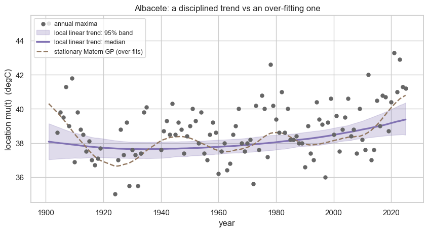

Line, ODE, and GP on one set of axes¶

The series in one figure. We refit the linear-location model and the energy-balance ODE and overlay their median $\mu(t)$ on the local-linear-trend band. Now that the GP is regularised, the three agree: a smooth rise of about a degree across the century, the GP merely flexing slightly where the ODE and line cannot.

z_lin = (yr - yr.mean()) / yr.std()
zc = jnp.asarray(z_lin)
def gev_lin(obs, zz):
    a = numpyro.sample("a", ndist.Normal(y_mean, 5.0))
    b = numpyro.sample("b", ndist.Normal(0.0, 2.0))
    ls = numpyro.sample("ls", ndist.Normal(np.log(y_std), 0.5))
    xi = numpyro.sample("xi", ndist.Normal(0.0, 0.25))
    numpyro.sample("obs", GEV(loc=a + b * zz, scale=jnp.exp(ls),
                              concentration=xi), obs=obs)
lin = MCMC(NUTS(gev_lin, target_accept_prob=0.99, init_strategy=init_to_median),
           num_warmup=800, num_samples=800, num_chains=2,
           chain_method="vectorized", progress_bar=False)
lin.run(jr.PRNGKey(2), y, zc)
plin = lin.get_samples()
mu_line = np.median(plin["a"]) + np.median(plin["b"]) * z_lin

t0, t1 = float(yr.min()), float(yr.max()); ts = jnp.asarray(yr, float); ALPHA = 2.0
def forcing(t):
    u = (t - t0) / (t1 - t0)
    return (jnp.exp(ALPHA * u) - 1.0) / (jnp.exp(ALPHA) - 1.0)
def integrate(beta, tau, tq):
    def vf(t, T, args): return (beta * forcing(t) - T) / tau
    sol = diffeqsolve(ODETerm(vf), Tsit5(), t0=t0, t1=t1, dt0=0.5, y0=0.0,
                      saveat=SaveAt(ts=tq), stepsize_controller=ConstantStepSize(),
                      max_steps=2000)
    return sol.ys
def gev_ode(obs):
    mu0 = numpyro.sample("mu0", ndist.Normal(y_mean, 5.0))
    beta = numpyro.sample("beta", ndist.Normal(0.0, 3.0))
    tau = numpyro.sample("tau", ndist.LogNormal(np.log(20.0), 0.8))
    ls = numpyro.sample("log_sigma", ndist.Normal(np.log(y_std), 0.5))
    xi = numpyro.sample("xi", ndist.Normal(0.0, 0.25))
    numpyro.sample("obs", GEV(loc=mu0 + integrate(beta, tau, ts),
                              scale=jnp.exp(ls), concentration=xi), obs=obs)
ode = MCMC(NUTS(gev_ode, target_accept_prob=0.95, init_strategy=init_to_median),
           num_warmup=800, num_samples=800, num_chains=2,
           chain_method="sequential", progress_bar=False)
ode.run(jr.PRNGKey(3), y)
pode = ode.get_samples()
mu_ode = np.median(pode["mu0"]) + np.asarray(
    integrate(np.median(pode["beta"]), np.median(pode["tau"]), ts))

fig, ax = plt.subplots(figsize=(10, 5))
ax.scatter(yr, y_np, color="0.55", s=22, zorder=3, label="annual maxima")
ax.fill_between(yr, mu_lo, mu_hi, color="#8172B3", alpha=0.20)
ax.plot(yr, mu_med, color="#8172B3", lw=2.6, label="GP / local linear trend")
ax.plot(yr, mu_ode, color="#C44E52", lw=2, ls="-.", label="ODE (NB11)")
ax.plot(yr, mu_line, color="#4C72B0", lw=2, ls="--", label="line (NB10)")
ax.set(xlabel="year", ylabel="location mu(t)  (degC)",
       title=f"{place}: three models of the warming trend, now in agreement")
ax.legend(loc="upper left", fontsize=9)
plt.show()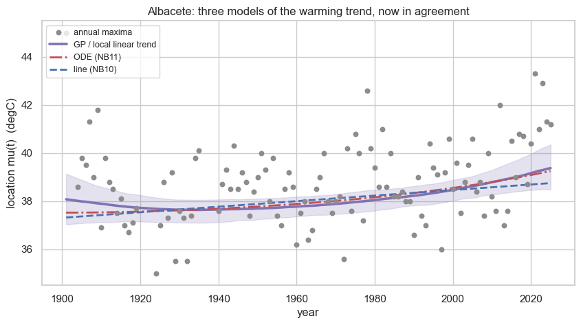

WAIC across the family¶

The scorecard. WAIC estimates out-of-sample fit; lower is better. The local-linear-trend GP still carries latent states, so its score is mildly optimistic — but, unlike the free Matérn GP (whose conditional WAIC plunges far below the rest by fitting the wiggles in-sample), the disciplined trend lands in a tight band with the line and ODE. Letting $\mu(t)$ move clearly helps; how you let it move barely matters here.

def waic(ll):
    S = ll.shape[0]
    lppd = logsumexp(ll, axis=0) - jnp.log(S)
    return float(-2.0 * (lppd.sum() - ll.var(axis=0).sum()))

def gev_stat(obs):
    mu = numpyro.sample("mu", ndist.Normal(y_mean, 5.0))
    sigma = numpyro.sample("sigma", ndist.HalfNormal(y_std))
    xi = numpyro.sample("xi", ndist.Normal(0.0, 0.25))
    numpyro.sample("obs", GEV(loc=mu, scale=sigma, concentration=xi), obs=obs)
stat = MCMC(NUTS(gev_stat, target_accept_prob=0.99, init_strategy=init_to_median),
            num_warmup=800, num_samples=800, num_chains=2,
            chain_method="vectorized", progress_bar=False)
stat.run(jr.PRNGKey(4), y)
pst = stat.get_samples()

ll_stat = gev_log_prob(y[None, :], pst["mu"][:, None], pst["sigma"][:, None], pst["xi"][:, None])
ll_line = gev_log_prob(y[None, :], plin["a"][:, None] + plin["b"][:, None] * zc[None, :],
                       jnp.exp(plin["ls"])[:, None], plin["xi"][:, None])
T_ode = jax.vmap(lambda b, ta: integrate(b, ta, ts))(pode["beta"], pode["tau"])
ll_ode = gev_log_prob(y[None, :], pode["mu0"][:, None] + T_ode,
                      jnp.exp(pode["log_sigma"])[:, None], pode["xi"][:, None])
f_all = jax.vmap(lambda s0, ss, zz: llt_trend(s0, ss, zz))(
    post["slope0"], post["sigma_s"], post["z"])
ll_gp = gev_log_prob(y[None, :], post["mu0"][:, None] + f_all,
                     jnp.exp(post["log_sigma"])[:, None], post["xi"][:, None])
f_mat = jax.vmap(lambda e, zz: matern32(e, 2.0, zz))(pmat["ell"], pmat["z2"])
ll_mat = gev_log_prob(y[None, :], pmat["mu0"][:, None] + f_mat,
                      jnp.exp(pmat["log_sigma"])[:, None], pmat["xi"][:, None])
tab = pd.DataFrame({"WAIC": [waic(ll_stat), waic(ll_line), waic(ll_ode),
                             waic(ll_gp), waic(ll_mat)]},
                   index=["stationary", "line (NB10)", "ODE (NB11)",
                          "GP local-linear", "GP stationary Matern"])
tab["dWAIC"] = tab["WAIC"] - tab["WAIC"].min()
print(tab.round(2).to_string())
print("\n(the stationary-Matern WAIC is the lowest, but that is the in-sample "
      "over-fitting flagged above — not a real predictive win.)")

                        WAIC  dWAIC
stationary            447.91  35.06
line (NB10)           443.21  30.35
ODE (NB11)            439.07  26.21
GP local-linear       436.42  23.56
GP stationary Matern  412.86   0.00

(the stationary-Matern WAIC is the lowest, but that is the in-sample over-fitting flagged above — not a real predictive win.)

Time-varying return levels¶

The return level rides the smooth trend. We read it at the GP location for the first and last years and place each maximum at its own-year climate, coloured by year — and because the trend no longer wiggles, the cloud now migrates cleanly from the early envelope up to the recent one.

mu0_m = float(np.median(post["mu0"]))
sig_m = float(np.exp(np.median(post["log_sigma"])))
xi_m = float(np.median(post["xi"]))
loc_year = mu0_m + np.median(f_draws, axis=0)
p_t = np.asarray(gev_survival(y, jnp.asarray(loc_year), sig_m, xi_m))
p_t = np.clip(p_t, 0.5 / n, None)
T_own = 1.0 / p_t
t_lo = max(1.02, float(T_own.min()))
periods = jnp.logspace(np.log10(t_lo), 3, 80)

jfirst = int(np.argmin(yr)); jlast = int(np.argmax(yr))
def rl_curve(jyear):
    locs = post["mu0"][sub] + f_draws[:, jyear]
    sig = jnp.exp(post["log_sigma"])[sub]; xi = post["xi"][sub]
    rl = jax.vmap(lambda i: GEV(loc=locs[i], scale=sig[i], concentration=xi[i])
                  .return_level(periods))(jnp.arange(locs.size))
    return np.asarray(rl)

fig, ax = plt.subplots(figsize=(8.8, 5))
for j, c, lab in [(jfirst, "#4C72B0", f"climate of {yr.min()}"),
                  (jlast, "#C44E52", f"climate of {yr.max()}")]:
    rl = rl_curve(j)
    med, lo, hi = (np.quantile(rl, q, 0) for q in (0.5, 0.025, 0.975))
    ax.fill_between(np.asarray(periods), lo, hi, color=c, alpha=0.16)
    ax.plot(np.asarray(periods), med, color=c, lw=2, label=lab)
sc = ax.scatter(T_own, y_np, c=yr, cmap="coolwarm", s=28, zorder=6,
                edgecolor="0.25", linewidth=0.3, label="observed maxima")
fig.colorbar(sc, ax=ax, pad=0.02).set_label("year of the maximum")
ax.set_xscale("log")
ax.set(xlabel="return period T (years)", ylabel=r"return level $z_T$ (degC)",
       title=f"{place}: return levels under the local-linear-trend GP")
ax.legend(loc="upper left")
plt.show()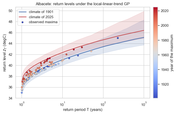

Extension: a trend on the scale, too¶

The same state-space machinery extends to a second local-linear trend on the log-scale, $\log\sigma(t)=s_0+g(t)$ , letting the spread of summer maxima drift as freely as the centre. We give it its own innovations and slope-diffusion and ask whether the data want it.

def gev_llt2(obs):
    mu0 = numpyro.sample("mu0", ndist.Normal(y_mean, 5.0))
    slope0 = numpyro.sample("slope0", ndist.Normal(0.0, 0.05))
    sig_s = numpyro.sample("sigma_s", ndist.HalfNormal(0.003))
    s0 = numpyro.sample("s0", ndist.Normal(np.log(y_std), 0.5))
    sslope0 = numpyro.sample("sslope0", ndist.Normal(0.0, 0.01))
    sig_g = numpyro.sample("sigma_g", ndist.HalfNormal(0.0010))
    xi = numpyro.sample("xi", ndist.Normal(0.0, 0.25))
    zf = numpyro.sample("zf", ndist.Normal(0, 1).expand([n - 1, 2]).to_event(2))
    zg = numpyro.sample("zg", ndist.Normal(0, 1).expand([n - 1, 2]).to_event(2))
    f = llt_trend(slope0, sig_s, zf)
    g = llt_trend(sslope0, sig_g, zg)
    numpyro.sample("obs", GEV(loc=mu0 + f, scale=jnp.exp(s0 + g),
                              concentration=xi), obs=obs)

mcmc2 = MCMC(NUTS(gev_llt2, target_accept_prob=0.95, init_strategy=init_to_median),
             num_warmup=1000, num_samples=1000, num_chains=2,
             chain_method="vectorized", progress_bar=False)
mcmc2.run(jr.PRNGKey(5), y)
post2 = mcmc2.get_samples()
g_draws = jax.vmap(lambda s0, ss, zz: llt_trend(s0, ss, zz))(
    post2["sslope0"][sub], post2["sigma_g"][sub], post2["zg"][sub])
sig_t = np.asarray(jnp.exp(post2["s0"][sub][:, None] + g_draws))
sig_rng = np.median(sig_t, 0)
f_all2 = jax.vmap(lambda s0, ss, zz: llt_trend(s0, ss, zz))(
    post2["slope0"], post2["sigma_s"], post2["zf"])
g_all2 = jax.vmap(lambda s0, ss, zz: llt_trend(s0, ss, zz))(
    post2["sslope0"], post2["sigma_g"], post2["zg"])
ll_gp2 = gev_log_prob(y[None, :], post2["mu0"][:, None] + f_all2,
                      jnp.exp(post2["s0"][:, None] + g_all2), post2["xi"][:, None])
print(f"sigma(t) spans {sig_rng.min():.2f}-{sig_rng.max():.2f} degC across the record")
print(f"WAIC: trend on mu only {waic(ll_gp):.1f}  |  trend on mu+sigma {waic(ll_gp2):.1f}")
print("scale trend " + ("helps" if waic(ll_gp2) < waic(ll_gp) - 2
      else "is not supported — the spread is effectively constant"))

sigma(t) spans 1.38-1.80 degC across the record
WAIC: trend on mu only 436.4  |  trend on mu+sigma 437.2
scale trend is not supported — the spread is effectively constant

Recap & series finale¶

We let the data shape the trend — but with a prior that defaults to a line. The local linear trend, an integrated random walk in state-space form ((2)), is the stochastic sibling of the previous notebook’s ODE and is walked in $O(n)$ via the Markov recursion ((3)). Crucially, it is the disciplined GP: a free stationary Matérn kernel over-fits a single short record, chasing multidecadal noise, while this prior bends only as much as the data buy.

With that discipline, the three trend models agree: a smooth warming of about a degree across the century, return levels today well above 1901’s, and a tail shape ξ the data place consistently across all of them. The line, the ODE, and the GP differ most where data are thinnest — the GP simply reports wider uncertainty there. The reassuring lesson is that the warming signal is robust to the model of the trend; the caution is that flexibility, unregularised, will manufacture structure that is not there.

The series. From a single GEV fit (The GEV distribution) we pooled across space (hierarchies and spatial GPs, NB04–09) and then let the parameters move through time at one station, three ways (NB10–12). The natural synthesis is a field that varies over space and time together — a spatio-temporal GP on the GEV parameters, the state-space trick of this notebook running along the time axis at every site of the spatial models. That is where a modern non-stationary extremes model lives.