SVGP + RFF NN kernel - Research Notebook

SVGP with a deep RFF kernel¶

The closing notebook in the pyrox SVGP series. So far we’ve kept the kernel fixed (RBF) and varied the inducing distribution — point-inducing in notebook 1, the same model mini-batched in notebook 2, spherical-harmonic in notebook 3. Now we keep the inducing distribution simple (point-inducing, $M = 30$ ) and replace the kernel with a deep-kernel construction.

The setup: a small MLP $\phi: \mathbb{R}^D \to \mathbb{R}^H$ warps the input space, and a random-Fourier-feature (RFF) projection of the warp produces a finite-dimensional kernel,

k(x, x') = \sigma^2 \, \psi(x)^\top \psi(x'), \qquad \psi(x) = \sqrt{\tfrac{2}{J}}\cos\!\bigl(W \phi(x) / \ell + b\bigr),

(1)

with $W \in \mathbb{R}^{H \times J}$ Gaussian, $b \in [0, 2\pi)^J$ uniform, and all of $\{\phi, W, b, \sigma, \ell\}$ trained jointly with the SVGP guide. The kernel is strictly PSD (it’s an inner product of features) and has rank at most $J$ , which is fine for $M \ll J$ .

Pyrox ships nine different RFF families in pyrox.nn._layers — RBF, Matérn, Laplace, arc-cosine, orthogonal, kitchen sinks, variational Fourier, HSGP — but for this notebook we hand-roll the RBF variant inside a custom Kernel subclass so the deep-kernel plumbing is fully explicit.

Background — when does an RBF need help?¶

The stationarity assumption¶

RBF kernels assume that the “right” notion of input similarity is Euclidean distance. Under one global lengthscale the prior covariance is the same function of $\|x - x'\|$ everywhere. That is a strong assumption — it fails whenever the generating process has direction-dependent or region-dependent smoothness.

Two common failure modes¶

Anisotropy. If the function is smooth in one direction and rough in another, a single $\ell$ smooths the rough direction too much or oscillates in the smooth one. ARD lengthscales fix this only when the principal axes align with the input axes.
Non-stationarity. If the effective lengthscale varies across the input space — a high-frequency patch near the origin and a slowly varying tail far away — a single global $\ell$ cannot match both regimes simultaneously.

Deep kernels, one sentence¶

An MLP is a universal function approximator; composing any stationary kernel with an MLP ( $k(\phi(x), \phi(x'))$ ) gives a kernel that can be non-stationary in the original input space while remaining stationary in the warped space — exactly the inductive bias that the SVGP ELBO will push toward whatever warp best explains the data.

Why RFF?¶

Two reasons. First, an RBF evaluated on a feature map has cost $\mathcal{O}(N M D)$ per training batch, where $D$ is the warp dimension; the RFF projection replaces that with $\mathcal{O}(N M J)$ where $J$ is a user-chosen truncation. Second, the features $\psi(x)$ are the same objects that SSGP and Bayesian-neural-field models expose — this notebook doubles as a bridge to pyrox’s pyrox.nn RFF zoo.

Setup¶

import equinox as eqx
import jax
import jax.numpy as jnp
import jax.random as jr
import matplotlib.pyplot as plt
import optax
from jaxtyping import Array, Float

from pyrox.gp import (
    GaussianLikelihood,
    Kernel,
    SparseGPPrior,
    WhitenedGuide,
    svgp_elbo,
)
from pyrox.gp._src.kernels import rbf_kernel

jax.config.update("jax_enable_x64", True)

/anaconda/lib/python3.13/site-packages/tqdm/auto.py:21: TqdmWarning: IProgress not found. Please update jupyter and ipywidgets. See https://ipywidgets.readthedocs.io/en/stable/user_install.html
  from .autonotebook import tqdm as notebook_tqdm

Data — a warped 2D target¶

Target function $y(x_1, x_2) = \sin\!\bigl(2\pi (x_1^2 - x_2)\bigr)$ on $[-1, 1]^2$ . The “effective” coordinate is the parabola $u = x_1^2 - x_2$ , so level sets of the target are parabolic ridges. A stationary RBF can’t represent the ridges cleanly with one lengthscale — the function looks highly oscillatory where $|x_1|$ is large and more gradual where $x_2$ dominates, a classic non-stationary pattern.

def f_true(X: Float[Array, "N 2"]) -> Float[Array, " N"]:
    return jnp.sin(2.0 * jnp.pi * (X[:, 0] ** 2 - X[:, 1]))


key = jr.PRNGKey(0)
key, key_X, key_noise = jr.split(key, 3)
N = 600
X_train = jr.uniform(key_X, (N, 2), minval=-1.0, maxval=1.0)
noise_std = 0.1
y_train = f_true(X_train) + noise_std * jr.normal(key_noise, (N,))

# Dense grid for plotting + evaluation.
G = 80
x1 = jnp.linspace(-1.0, 1.0, G)
x2 = jnp.linspace(-1.0, 1.0, G)
X1_grid, X2_grid = jnp.meshgrid(x1, x2, indexing="xy")
X_grid = jnp.stack([X1_grid.ravel(), X2_grid.ravel()], axis=-1)
y_grid_true = f_true(X_grid).reshape(G, G)

fig, ax = plt.subplots(figsize=(6, 5))
mesh = ax.pcolormesh(X1_grid, X2_grid, y_grid_true, cmap="RdBu_r", vmin=-1.0, vmax=1.0, shading="auto")
ax.scatter(X_train[:, 0], X_train[:, 1], s=3, alpha=0.3, color="k")
fig.colorbar(mesh, ax=ax, label="f(x)")
ax.set_xlabel("$x_1$")
ax.set_ylabel("$x_2$")
ax.set_title("Target $f(x) = \\sin(2\\pi(x_1^2 - x_2))$ with 600 training points")
ax.set_aspect("equal")
plt.show()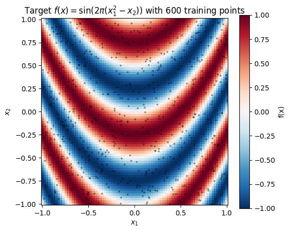

Level sets of $f$ are the parabolas $x_1^2 - x_2 = c$ (plus any integer shift due to the $\sin$ ). A stationary RBF wants axis-aligned, constant-lengthscale isolines — the mismatch is severe.

Kernels — RBF baseline and the deep RFF variant¶

class RBFLite(Kernel, eqx.Module):
    """Pure-equinox RBF — the baseline from notebooks 1 and 2."""

    log_variance: Float[Array, ""]
    log_lengthscale: Float[Array, ""]

    @classmethod
    def init(cls, variance: float = 1.0, lengthscale: float = 1.0) -> "RBFLite":
        return cls(
            log_variance=jnp.log(jnp.asarray(variance)),
            log_lengthscale=jnp.log(jnp.asarray(lengthscale)),
        )

    @property
    def variance(self) -> Float[Array, ""]:
        return jnp.exp(self.log_variance)

    @property
    def lengthscale(self) -> Float[Array, ""]:
        return jnp.exp(self.log_lengthscale)

    def __call__(
        self,
        X1: Float[Array, "N1 D"],
        X2: Float[Array, "N2 D"],
    ) -> Float[Array, "N1 N2"]:
        return rbf_kernel(X1, X2, self.variance, self.lengthscale)

    def diag(self, X: Float[Array, "N D"]) -> Float[Array, " N"]:
        return self.variance * jnp.ones(X.shape[0], dtype=X.dtype)

The deep RFF kernel carries trainable mlp, W, b, and log-scales. The MLP is a plain equinox.nn.MLP (two hidden layers, 32 units, tanh activation); its parameters are equinox leaves and train via the same optax.adam loop as the other scalars.

class DeepRFFKernel(Kernel, eqx.Module):
    """Deep kernel:  k(x, x') = σ² ⟨ψ(x), ψ(x')⟩  where  ψ = RFF ∘ MLP."""

    mlp: eqx.nn.MLP
    W: Float[Array, "H J"]
    b: Float[Array, " J"]
    log_variance: Float[Array, ""]
    log_feature_lengthscale: Float[Array, ""]

    @classmethod
    def init(
        cls,
        in_dim: int,
        hidden_dim: int,
        num_features: int,
        *,
        key: jr.PRNGKey,
        mlp_width: int = 32,
        mlp_depth: int = 2,
        variance: float = 1.0,
        feature_lengthscale: float = 1.0,
    ) -> "DeepRFFKernel":
        k_mlp, k_W, k_b = jr.split(key, 3)
        mlp = eqx.nn.MLP(
            in_size=in_dim,
            out_size=hidden_dim,
            width_size=mlp_width,
            depth=mlp_depth,
            activation=jax.nn.tanh,
            key=k_mlp,
        )
        W = jr.normal(k_W, (hidden_dim, num_features))
        b = jr.uniform(k_b, (num_features,)) * 2.0 * jnp.pi
        return cls(
            mlp=mlp,
            W=W,
            b=b,
            log_variance=jnp.log(jnp.asarray(variance)),
            log_feature_lengthscale=jnp.log(jnp.asarray(feature_lengthscale)),
        )

    def _features(self, X: Float[Array, "N D"]) -> Float[Array, "N J"]:
        phi = jax.vmap(self.mlp)(X)
        z = phi @ self.W / jnp.exp(self.log_feature_lengthscale) + self.b
        return jnp.sqrt(2.0 / self.W.shape[1]) * jnp.cos(z)

    def __call__(
        self,
        X1: Float[Array, "N1 D"],
        X2: Float[Array, "N2 D"],
    ) -> Float[Array, "N1 N2"]:
        return jnp.exp(self.log_variance) * self._features(X1) @ self._features(X2).T

    def diag(self, X: Float[Array, "N D"]) -> Float[Array, " N"]:
        psi = self._features(X)
        return jnp.exp(self.log_variance) * jnp.sum(psi * psi, axis=-1)


class TrainableGaussianLikelihood(eqx.Module):
    log_noise_var: Float[Array, ""]

    @classmethod
    def init(cls, noise_var: float = 0.1) -> "TrainableGaussianLikelihood":
        return cls(log_noise_var=jnp.log(jnp.asarray(noise_var)))

    def materialise(self) -> GaussianLikelihood:
        return GaussianLikelihood(noise_var=jnp.exp(self.log_noise_var))

Shared training loop¶

Same ELBO, same optimiser — only the kernel inside prior changes between the two runs.

Params = tuple


def neg_elbo(params: Params, X: Float[Array, "N D"], y: Float[Array, " N"]) -> Float[Array, ""]:
    prior_p, guide_p, lik_p = params
    return -svgp_elbo(prior_p, guide_p, lik_p.materialise(), X, y)


def train(
    prior: SparseGPPrior,
    guide: WhitenedGuide,
    lik_w: TrainableGaussianLikelihood,
    X: Float[Array, "N D"],
    y: Float[Array, " N"],
    *,
    lr: float = 1e-2,
    n_steps: int = 3000,
) -> tuple[Params, list[float]]:
    params = (prior, guide, lik_w)
    # Gradient clipping keeps the deep-kernel loss smooth — without it, Adam
    # occasionally lands a step that pushes the MLP into a flat region of the
    # cos-feature map and the ELBO spikes before recovering.
    optimiser = optax.chain(optax.clip_by_global_norm(1.0), optax.adam(lr))
    opt_state = optimiser.init(eqx.filter(params, eqx.is_inexact_array))

    @eqx.filter_jit
    def step(params, opt_state):
        loss, grads = eqx.filter_value_and_grad(neg_elbo)(params, X, y)
        updates, opt_state = optimiser.update(grads, opt_state, params)
        return eqx.apply_updates(params, updates), opt_state, loss

    losses: list[float] = []
    for _ in range(n_steps):
        params, opt_state, loss = step(params, opt_state)
        losses.append(float(loss))
    return params, losses

Baseline — standard SVGP with RBF kernel¶

$M = 30$ inducing points on a $6 \times 5$ grid covering the domain.

M = 30
gx, gy = jnp.meshgrid(jnp.linspace(-0.8, 0.8, 6), jnp.linspace(-0.8, 0.8, 5), indexing="xy")
Z_init = jnp.stack([gx.ravel(), gy.ravel()], axis=-1)

prior_rbf = SparseGPPrior(
    kernel=RBFLite.init(variance=1.0, lengthscale=0.3),
    Z=Z_init,
    jitter=1e-4,
)
guide_rbf = WhitenedGuide.init(num_inducing=M)
lik_rbf = TrainableGaussianLikelihood.init(noise_var=noise_std**2)

(prior_rbf_fit, guide_rbf_fit, lik_rbf_fit), losses_rbf = train(
    prior_rbf, guide_rbf, lik_rbf, X_train, y_train
)
print(f"RBF     final -ELBO = {losses_rbf[-1]:.3f}")
print(f"        variance    = {float(prior_rbf_fit.kernel.variance):.3f}")
print(f"        lengthscale = {float(prior_rbf_fit.kernel.lengthscale):.3f}")
print(f"        noise std   = {float(jnp.exp(0.5 * lik_rbf_fit.log_noise_var)):.3f}  (truth {noise_std})")

RBF     final -ELBO = 283.729
        variance    = 0.215
        lengthscale = 0.250
        noise std   = 0.293  (truth 0.1)

Deep RFF — same scaffold, swapped kernel¶

$J = 256$ Fourier features, hidden width 8 in the MLP output, initial feature lengthscale 0.5. Deep kernels have a noticeably harder loss landscape than the RBF baseline (more parameters, trigonometric nonlinearity in the features), so we drop the learning rate to 1e-2 and train for 3000 steps. With the stock 5e-2 / 1200 settings the MLP doesn’t have time to learn a useful warp and the deep kernel ends up worse than the RBF — a reminder that expressive priors are only useful when the optimiser can reach them.

prior_deep = SparseGPPrior(
    kernel=DeepRFFKernel.init(
        in_dim=2,
        hidden_dim=8,
        num_features=256,
        key=jr.PRNGKey(7),
        mlp_width=32,
        mlp_depth=2,
        variance=1.0,
        feature_lengthscale=0.5,
    ),
    Z=Z_init,
    jitter=1e-4,
)
guide_deep = WhitenedGuide.init(num_inducing=M)
lik_deep = TrainableGaussianLikelihood.init(noise_var=noise_std**2)

(prior_deep_fit, guide_deep_fit, lik_deep_fit), losses_deep = train(
    prior_deep, guide_deep, lik_deep, X_train, y_train
)
print(f"DeepRFF final -ELBO = {losses_deep[-1]:.3f}")
print(f"        variance    = {float(jnp.exp(prior_deep_fit.kernel.log_variance)):.3f}")
print(f"        feat scale  = {float(jnp.exp(prior_deep_fit.kernel.log_feature_lengthscale)):.3f}")
print(f"        noise std   = {float(jnp.exp(0.5 * lik_deep_fit.log_noise_var)):.3f}  (truth {noise_std})")

DeepRFF final -ELBO = -493.297
        variance    = 0.444
        feat scale  = 0.843
        noise std   = 0.101  (truth 0.1)

Loss curves — side by side¶

fig, ax = plt.subplots(figsize=(10, 3.5))
ax.plot(losses_rbf, color="C0", lw=1.5, label="RBF baseline")
ax.plot(losses_deep, color="C3", lw=1.5, label="Deep RFF")
ax.set_xlabel("step")
ax.set_ylabel("−ELBO")
ax.set_yscale("symlog", linthresh=10.0)
ax.set_title("SVGP training — RBF vs deep RFF")
ax.grid(alpha=0.3, which="both")
ax.legend()
plt.show()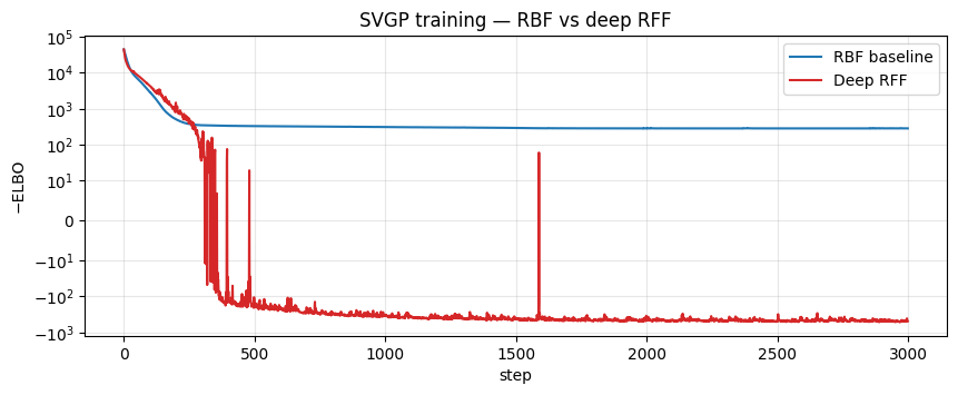

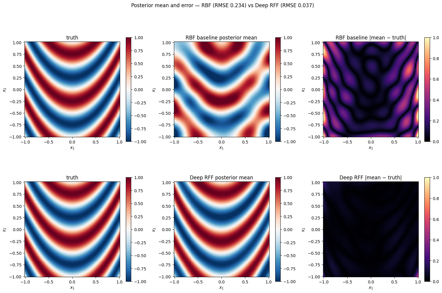
Posterior comparison¶

Evaluate both posteriors on the $80 \times 80$ grid and plot mean + |mean − truth| error maps side-by-side.

def posterior_mean(prior_fit, guide_fit, X_eval):
    K_zz_op, K_xz, K_xx_diag = prior_fit.predictive_blocks(X_eval)
    f_loc, _ = guide_fit.predict(K_xz, K_zz_op, K_xx_diag)
    return (f_loc + prior_fit.mean(X_eval)).reshape(G, G)


mean_rbf = posterior_mean(prior_rbf_fit, guide_rbf_fit, X_grid)
mean_deep = posterior_mean(prior_deep_fit, guide_deep_fit, X_grid)
err_rbf = jnp.abs(mean_rbf - y_grid_true)
err_deep = jnp.abs(mean_deep - y_grid_true)

rmse_rbf = float(jnp.sqrt(jnp.mean((mean_rbf - y_grid_true) ** 2)))
rmse_deep = float(jnp.sqrt(jnp.mean((mean_deep - y_grid_true) ** 2)))
print(f"grid RMSE (RBF)     = {rmse_rbf:.3f}")
print(f"grid RMSE (DeepRFF) = {rmse_deep:.3f}")
print(f"noise-std baseline  = {noise_std:.3f}  (a perfect model would roughly match this)")

fig, axes = plt.subplots(2, 3, figsize=(15, 10))
for row, (name, mean_pred, err) in enumerate([
    ("RBF baseline", mean_rbf, err_rbf),
    ("Deep RFF", mean_deep, err_deep),
]):
    for col, (field, title, vmin, vmax, cmap) in enumerate([
        (y_grid_true, "truth", -1.0, 1.0, "RdBu_r"),
        (mean_pred, f"{name} posterior mean", -1.0, 1.0, "RdBu_r"),
        (err, f"{name} |mean − truth|", 0.0, 1.0, "magma"),
    ]):
        ax = axes[row, col]
        mesh = ax.pcolormesh(X1_grid, X2_grid, field, cmap=cmap, vmin=vmin, vmax=vmax, shading="auto")
        fig.colorbar(mesh, ax=ax, shrink=0.75)
        ax.set_aspect("equal")
        ax.set_xlabel("$x_1$")
        ax.set_ylabel("$x_2$")
        ax.set_title(title)
fig.suptitle(f"Posterior mean and error — RBF (RMSE {rmse_rbf:.3f}) vs Deep RFF (RMSE {rmse_deep:.3f})", y=1.01)
plt.tight_layout()
plt.show()

grid RMSE (RBF)     = 0.234
grid RMSE (DeepRFF) = 0.037
noise-std baseline  = 0.100  (a perfect model would roughly match this)

The learned warp¶

What does the MLP do to the input space? Pass a uniform $x$ -grid through kernel.mlp and scatter the result — this is the geometry the downstream RFF layer actually sees. A pair of adjacent test points whose true targets differ should be pushed apart by the warp; a pair with similar targets should be pulled together.

phi_grid = jax.vmap(prior_deep_fit.kernel.mlp)(X_grid)

# Colour each warped point by its true target value, so the visual is
# "similar colours cluster" iff the warp has learned the right metric.
target_colour = y_grid_true.ravel()

fig, axes = plt.subplots(1, 2, figsize=(11, 4.5))
axes[0].scatter(
    X_grid[:, 0],
    X_grid[:, 1],
    c=target_colour,
    cmap="RdBu_r",
    vmin=-1.0,
    vmax=1.0,
    s=6,
)
axes[0].set_xlabel("$x_1$")
axes[0].set_ylabel("$x_2$")
axes[0].set_title("Input space — coloured by target value")
axes[0].set_aspect("equal")

# Show the first two principal axes of phi(X_grid) — this is the 4-dim
# warp projected to 2D for visualisation only.
phi_centred = phi_grid - phi_grid.mean(axis=0, keepdims=True)
_, _, Vt = jnp.linalg.svd(phi_centred, full_matrices=False)
phi_2d = phi_centred @ Vt[:2].T
axes[1].scatter(
    phi_2d[:, 0],
    phi_2d[:, 1],
    c=target_colour,
    cmap="RdBu_r",
    vmin=-1.0,
    vmax=1.0,
    s=6,
)
axes[1].set_xlabel("φ PC1")
axes[1].set_ylabel("φ PC2")
axes[1].set_title("Warped space φ(x) — first two PCs")
axes[1].set_aspect("equal")
plt.tight_layout()
plt.show()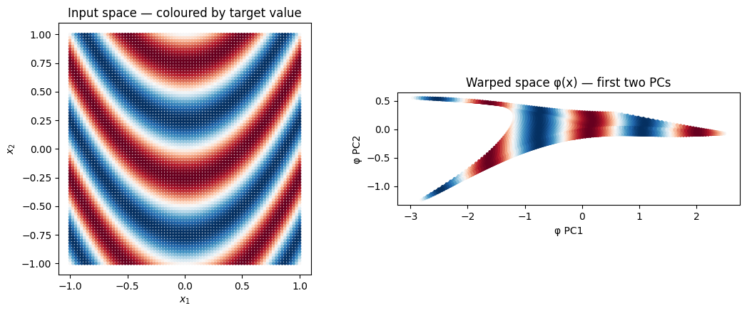

In the left panel, neighbouring points can have wildly different colours — the parabolic level sets of the target tangle any local Euclidean metric. In the right panel the warp should re-layer those same points so that colour correlates with position: same-coloured points cluster, gradients become smooth. That is the geometry the SVGP kernel now operates on, and it is the reason the deep-RFF posterior mean matches the truth where the RBF’s one-lengthscale smoother cannot.

Summary¶

Four SVGPs, one ELBO, one training loop — only the kernel or batching strategy changes between notebooks. Point-inducing RBF (notebook 1), mini-batched training (notebook 2), spherical-harmonic inducing (notebook 3), deep RFF kernel (this notebook).
Deep kernels buy expressive power when the input geometry is non-stationary, at the cost of more parameters and a harder loss landscape — watch for overfitting, especially with small $N$ .
The RFF projection keeps the kernel matrix low-rank ( $J$ features) while the MLP does the heavy lifting; bumping $J$ and hidden width independently gives two orthogonal dials for capacity.

Where to go next. Pyrox ships eight other RFF variants in pyrox.nn._layers (Matérn RFF, Laplace RFF, arc-cosine features, orthogonal random features, kitchen sinks, HSGP features, variational Fourier features) — each is a drop-in replacement for the cos(Wx + b) basis used above. The pyrox.gp.FourierInducingFeatures family lets you combine a deep kernel with inter-domain inducing features for the best-of-both-worlds recipe on bounded domains; pair with NaturalGuide + ConjugateVI for natural-gradient training, or with DistLikelihood for Bernoulli/Poisson SVGPs.