The Arakawa C-Grid - somax: Simple Ocean Models in JAX

Every somax model discretises its fields on a staggered Arakawa C-grid, supplied by finitevolX. Staggering is not an implementation detail — it is the choice that makes the discrete operators mimic the continuous ones (a discrete gradient that lands exactly where the next operator needs it, a divergence that is genuinely the adjoint of the gradient). This chapter shows where each field lives, how ghost cells frame the physical interior, and why the layout matters Arakawa & Lamb (1977)Durran (2010).

What you will learn

The four stagger positions (T, U, V, X) and the half-index convention that places them
How finitevolX frames the interior with a one-cell ghost halo
How to construct a grid and create correctly-shaped staggered fields

Why stagger?¶

Consider the rotating shallow-water system, the prototype for the ocean models in this book Vallis (2017). Mass conservation couples the layer thickness $h$ to the divergence of the transport,

\partial_t h + \nabla\cdot(h\,\mathbf{u}) = 0,

(1)

while the momentum balance couples the velocity $\mathbf{u}=(u,v)$ to the pressure gradient,

\partial_t \mathbf{u} + (f\,\hat{\mathbf{z}}\times\mathbf{u}) = -g\,\nabla h .

(2)

On a collocated grid (all variables at the cell centre), the pressure gradient $\nabla h$ in (2) needs a centred two-cell stencil, which is blind to the $2\Delta x$ checkerboard mode — pressure and velocity decouple and spurious grid-scale noise grows. The C-grid cure is to place $u$ and $v$ on the cell faces, half a cell from the pressure point, so the gradient in (2) and the divergence in (1) both become compact one-cell differences that see every mode Arakawa & Lamb (1977).

The four stagger positions¶

A 2-D C-grid cell carries its variables at four distinct locations, named by the somax/finitevolX convention in Table 1. Writing the cell index as $[j, i]$ (row $j$ , column $i$ ) and the cell spacing as $(\Delta x, \Delta y)$ , the half-index offsets are:

Table 1:Stagger positions on the Arakawa C-grid. The index $[j,i]$ labels the south-west corner of the stencil neighbourhood (the “same-index” rule).

Symbol	Name	Location	Position of $[j,i]$	Typical field
`T`	cell centre	tracer point	$(i\,\Delta x,\; j\,\Delta y)$	thickness $h$ , pressure
`U`	east face	x-velocity point	$((i+\tfrac12)\,\Delta x,\; j\,\Delta y)$	zonal velocity $u$
`V`	north face	y-velocity point	$(i\,\Delta x,\; (j+\tfrac12)\,\Delta y)$	meridional velocity $v$
`X`	north-east corner	vorticity point	$((i+\tfrac12)\,\Delta x,\; (j+\tfrac12)\,\Delta y)$	vorticity $\zeta$ , PV $q$

The placement is exactly what the equations want: $u$ sits where $\partial_x h$ is naturally defined (between two T-points), and the vorticity $\zeta = \partial_x v - \partial_y u$ lands cleanly at the corner where the circulation around a cell is measured.

Constructing a grid¶

finitevolX exposes the C-grid through CartesianGrid2D. The from_interior factory is the idiomatic constructor: you give it the number of physical (interior) cells and the domain size, and it computes the spacing and adds the ghost halo.

import warnings

warnings.filterwarnings("ignore", message=r".*IProgress.*")

import importlib.util
from pathlib import Path

import finitevolx as fvx
import jax.numpy as jnp
import matplotlib.pyplot as plt
import numpy as np

try:
    from IPython import get_ipython

    ipython = get_ipython()
except ImportError:
    ipython = None

if ipython is not None and importlib.util.find_spec("watermark") is not None:
    ipython.run_line_magic("load_ext", "watermark")
    ipython.run_line_magic("watermark", "-v -m -p numpy,jax,finitevolx,somax")
else:
    print("watermark extension not installed; skipping reproducibility readout.")

watermark extension not installed; skipping reproducibility readout.

nx_interior = ny_interior = 16
grid = fvx.CartesianGrid2D.from_interior(
    nx_interior=nx_interior, ny_interior=ny_interior, Lx=1.0, Ly=1.0
)
print(f"interior cells : {nx_interior} x {ny_interior}")
print(
    f"full grid      : Nx={grid.Nx} x Ny={grid.Ny}  (interior + 1 ghost cell per side)"
)
print(f"spacing        : dx={grid.dx:.4f}, dy={grid.dy:.4f}")

interior cells : 16 x 16
full grid      : Nx=18 x Ny=18  (interior + 1 ghost cell per side)
spacing        : dx=0.0625, dy=0.0625

Ghost cells frame the interior¶

finitevolX surrounds the $n_x \times n_y$ physical cells with a one-cell ghost halo, so the stored arrays are $(n_y+2)\times(n_x+2)$ . The ghost cells hold the boundary-condition values (next chapter); every diagnostic and conserved integral in somax is taken over the interior slice [1:-1, 1:-1] to exclude them. All four stagger types share this same full shape — only their physical interpretation differs.

Ny, Nx = grid.Ny, grid.Nx
h = jnp.zeros((Ny, Nx))  # T-point: thickness / pressure
u = jnp.zeros((Ny, Nx))  # U-point: zonal velocity
v = jnp.zeros((Ny, Nx))  # V-point: meridional velocity
q = jnp.zeros((Ny, Nx))  # X-point: vorticity / PV

interior = (slice(1, -1), slice(1, -1))
print(f"stored field shape   : {h.shape}")
print(
    f"interior field shape : {h[interior].shape}  (the {nx_interior}x{ny_interior} physical cells)"
)

stored field shape   : (18, 18)
interior field shape : (16, 16)  (the 16x16 physical cells)

Visualising the stagger¶

Figure 1 overlays the four stagger positions for a single cell. The tracer point T anchors the cell; U/V sit on the east/north faces half a cell away; the vorticity point X sits at the north-east corner. This is the geometry that makes the discrete gradient, divergence, and curl land exactly where the next operator consumes them (next chapter).

# The notebook executes with cwd = content/tutorials/, and figures are
# referenced as ../images/<name>/ — i.e. content/images/<name>/.
IMG_DIR = Path.cwd().parent / "images" / "arakawa_cgrid"
IMG_DIR.mkdir(parents=True, exist_ok=True)

fig, ax = plt.subplots(figsize=(7, 7))
# Draw a 3x3 block of cells.
for k in range(4):
    ax.axhline(k, color="0.8", lw=1)
    ax.axvline(k, color="0.8", lw=1)
# Stagger markers for the cells.
tc, uc, vc, xc = [], [], [], []
for j in range(3):
    for i in range(3):
        tc.append((i + 0.5, j + 0.5))  # centre
        uc.append((i + 1.0, j + 0.5))  # east face
        vc.append((i + 0.5, j + 1.0))  # north face
        xc.append((i + 1.0, j + 1.0))  # NE corner
for pts, marker, label, color in [
    (tc, "o", "T  (h, pressure)", "C0"),
    (uc, ">", "U  (u)", "C1"),
    (vc, "^", "V  (v)", "C2"),
    (xc, "s", "X  (vorticity, PV)", "C3"),
]:
    arr = np.array(pts)
    ax.scatter(
        arr[:, 0], arr[:, 1], marker=marker, s=90, color=color, label=label, zorder=3
    )
ax.set(
    xlim=(-0.2, 3.2),
    ylim=(-0.2, 3.2),
    xlabel="x  (cell index i)",
    ylabel="y  (cell index j)",
    title="Arakawa C-grid stagger positions",
    aspect="equal",
)
ax.legend(loc="upper left", bbox_to_anchor=(1.02, 1.0), frameon=False)
fig.tight_layout()
fig.savefig(IMG_DIR / "stagger_positions.png", dpi=110, bbox_inches="tight")
plt.show()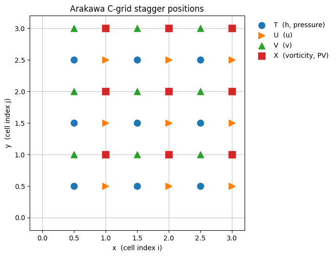

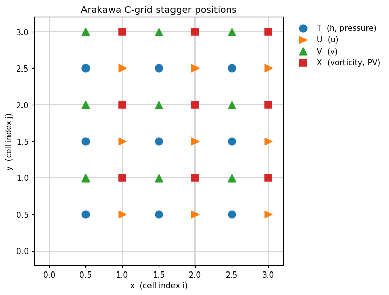
The four Arakawa C-grid stagger positions over a 3×3 block of cells. Tracer
quantities (T) sit at cell centres; velocities (U, V) on the east and
north faces; vorticity / potential vorticity (X) at the north-east corners. — Figure 1:The four Arakawa C-grid stagger positions over a 3×3 block of cells. Tracer quantities (`T`) sit at cell centres; velocities (`U`, `V`) on the east and north faces; vorticity / potential vorticity (`X`) at the north-east corners.

Summary¶

somax fields live on a staggered Arakawa C-grid: T (centre), U/V (faces), X (corner) — see Table 1 and Figure 1.
Staggering makes the pressure gradient in (2) and the divergence in (1) compact, mode-aware operators — the original motivation of Arakawa & Lamb (1977).
CartesianGrid2D.from_interior(...) builds the grid; the stored arrays carry a one-cell ghost halo, and diagnostics use the [1:-1, 1:-1] interior slice.

The next chapter, discrete operators, shows how the staggering lets Difference2D map fields between these positions to build gradients, divergences, and the vorticity.

References¶

Arakawa, A., & Lamb, V. R. (1977). Computational design of the basic dynamical processes of the UCLA general circulation model. Methods in Computational Physics, 17, 173–265.
Durran, D. R. (2010). Numerical Methods for Fluid Dynamics: With Applications to Geophysics (2nd ed., Vol. 32). Springer. 10.1007/978-1-4419-6412-0
Vallis, G. K. (2017). Atmospheric and oceanic fluid dynamics.