Discrete Operators - somax: Simple Ocean Models in JAX

With fields placed on the staggered grid from the previous chapter, the differential operators of fluid dynamics become finite differences and averages that move fields between stagger positions. This chapter walks through the four operator families finitevolX provides — differences, interpolations, advection, and the Laplacian — and shows each one mapping a field from one set of grid points to another Durran (2010)LeVeque (2002).

What you will learn

How Difference2D builds gradients, divergence, and curl as stagger-changing differences
How Interpolation2D averages fields between stagger positions
How Advection2D reconstructs fluxes with upwind / WENO schemes
How the Laplacian assembles into the elliptic operators the models invert

The stagger-changing rule¶

The defining feature of C-grid operators is that a derivative changes the stagger. A centred difference of a T-point field along $x$ naturally lives on the U-points half a cell away:

\big(\partial_x h\big)_{j,\,i+\frac12} \;\approx\; \frac{h_{j,i+1} - h_{j,i}}{\Delta x},

(1)

which is exactly the T → U map. Likewise $\partial_y$ of a T-field lands on V-points (T → V). The divergence of a velocity reverses this — it consumes face-staggered fluxes and returns a centred tendency,

\big(\nabla\cdot\mathbf{u}\big)_{j,i} \;\approx\; \frac{u_{j,\,i+\frac12} - u_{j,\,i-\frac12}}{\Delta x} + \frac{v_{j+\frac12,\,i} - v_{j-\frac12,\,i}}{\Delta y},

(2)

i.e. (U, V) → T. Because the same face values that the divergence consumes are the ones the gradient produces, the discrete divergence is the negative adjoint of the discrete gradient — the property that gives C-grid schemes their clean energy budgets Arakawa & Lamb (1977).

import warnings

warnings.filterwarnings("ignore", message=r".*IProgress.*")

import importlib.util
from pathlib import Path

import finitevolx as fvx
import jax.numpy as jnp
import matplotlib.pyplot as plt

try:
    from IPython import get_ipython

    ipython = get_ipython()
except ImportError:
    ipython = None

if ipython is not None and importlib.util.find_spec("watermark") is not None:
    ipython.run_line_magic("load_ext", "watermark")
    ipython.run_line_magic("watermark", "-v -m -p numpy,jax,finitevolx,somax")
else:
    print("watermark extension not installed; skipping reproducibility readout.")

watermark extension not installed; skipping reproducibility readout.

Setup: a smooth test field¶

We build a 64×64 grid and a smooth, analytically-differentiable test field $\psi(x,y) = \sin(2\pi x)\cos(2\pi y)$ so we can compare the discrete operators against their exact continuous counterparts.

grid = fvx.CartesianGrid2D.from_interior(nx_interior=64, ny_interior=64, Lx=1.0, Ly=1.0)
diff = fvx.Difference2D(grid=grid, mask=None)
interp = fvx.Interpolation2D(grid=grid, mask=None)
advection = fvx.Advection2D(grid=grid, mask=None)

x = jnp.linspace(0.0, 1.0, grid.Nx)
y = jnp.linspace(0.0, 1.0, grid.Ny)
xx, yy = jnp.meshgrid(x, y)
psi = jnp.sin(2 * jnp.pi * xx) * jnp.cos(2 * jnp.pi * yy)
print("test field psi:", psi.shape)

test field psi: (66, 66)

Differences: gradient, divergence, curl¶

Difference2D names each method by the stagger map it performs, so the code reads like (1)–(2). The exact $x$ -derivative of $\psi$ is $2\pi\cos(2\pi x)\cos(2\pi y)$ ; the discrete diff_x_T_to_U should reproduce it (up to the half-cell shift and truncation error).

dpsi_dx = diff.diff_x_T_to_U(psi)  # T -> U
dpsi_dy = diff.diff_y_T_to_V(psi)  # T -> V

# A divergence of a (u, v) pair returns to T-points.
u = diff.diff_x_T_to_U(psi)
v = diff.diff_y_T_to_V(psi)
div = diff.divergence(u, v)  # (U, V) -> T

# Curl (relative vorticity) of a velocity lands on the corner X-points.
zeta = diff.curl(u, v)  # (U, V) -> X

# Laplacian maps T -> T (used by the elliptic solvers, last section).
lap = diff.laplacian(psi)

for name, field in [
    ("diff_x_T_to_U", dpsi_dx),
    ("diff_y_T_to_V", dpsi_dy),
    ("divergence (U,V->T)", div),
    ("curl (U,V->X)", zeta),
    ("laplacian (T->T)", lap),
]:
    print(f"{name:24s}: shape {field.shape}")

diff_x_T_to_U           : shape (66, 66)
diff_y_T_to_V           : shape (66, 66)
divergence (U,V->T)     : shape (66, 66)
curl (U,V->X)           : shape (66, 66)
laplacian (T->T)        : shape (66, 66)

Figure 1 shows the field and its discrete $x$ -derivative side by side with the exact derivative. The discrete operator tracks the analytic one across the interior; the agreement is the evidence that the stagger map in (1) is faithful.

IMG_DIR = Path.cwd().parent / "images" / "operators"
IMG_DIR.mkdir(parents=True, exist_ok=True)

s = (slice(1, -1), slice(1, -1))
exact_dx = 2 * jnp.pi * jnp.cos(2 * jnp.pi * xx) * jnp.cos(2 * jnp.pi * yy)

fig, axes = plt.subplots(1, 3, figsize=(18, 5))
im0 = axes[0].pcolormesh(psi[s], cmap="RdBu_r")
axes[0].set(title=r"$\psi = \sin(2\pi x)\cos(2\pi y)$")
fig.colorbar(im0, ax=axes[0])
im1 = axes[1].pcolormesh(dpsi_dx[s], cmap="RdBu_r")
axes[1].set(title=r"discrete $\partial_x \psi$  (T$\to$U)")
fig.colorbar(im1, ax=axes[1])
im2 = axes[2].pcolormesh(exact_dx[s], cmap="RdBu_r")
axes[2].set(title=r"exact $\partial_x \psi$")
fig.colorbar(im2, ax=axes[2])
fig.tight_layout()
fig.savefig(IMG_DIR / "difference_x.png", dpi=110, bbox_inches="tight")
plt.show()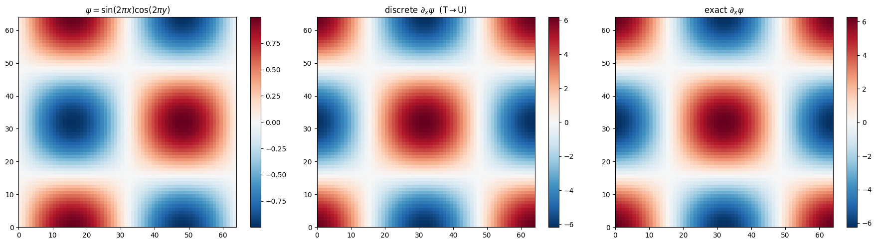

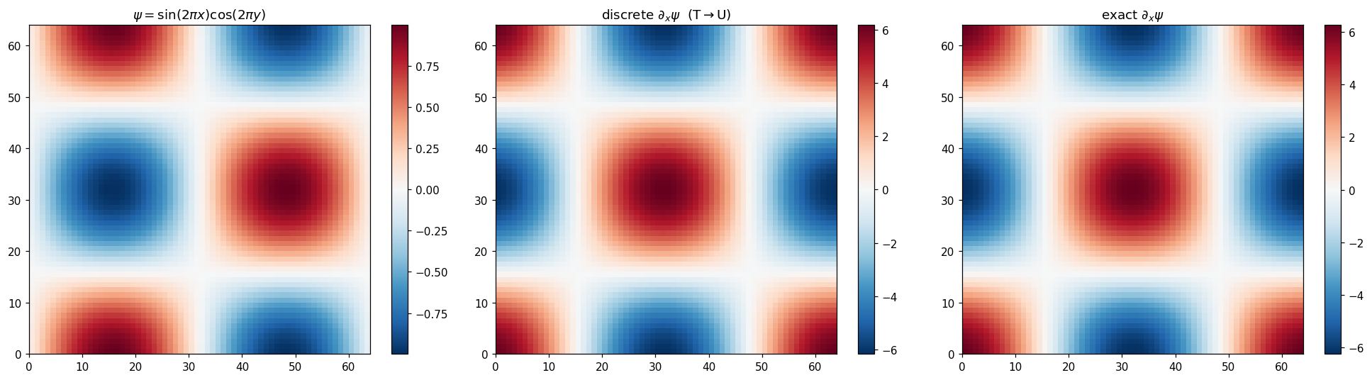
A smooth test field (left), its discrete x-derivative from
diff_x_T_to_U (centre), and the exact analytic derivative (right). The
discrete C-grid difference reproduces the continuous gradient across the
interior. — Figure 1:A smooth test field (left), its discrete $x$ -derivative from `diff_x_T_to_U` (centre), and the exact analytic derivative (right). The discrete C-grid difference reproduces the continuous gradient across the interior.

Interpolations: moving between stagger positions¶

Many terms mix fields from different stagger positions — the mass flux $h\,u$ needs $h$ (a T-field) evaluated at the U-points where $u$ lives. Interpolation2D provides the averaging maps, named by the same source-to-target convention as the differences. The methods are summarised in Table 1.

Table 1:A representative set of Interpolation2D averaging maps. Every map is a local average; the name encodes the source-to-target stagger.

Method	Map	Use
`T_to_U`, `T_to_V`	centre to face	thickness at velocity points (mass flux $h\,u$ )
`U_to_T`, `V_to_T`	face to centre	kinetic energy $\tfrac12(u^2+v^2)$ at T
`T_to_X`	centre to corner	thickness at the vorticity point (potential vorticity)
`X_to_U`, `X_to_V`	corner to face	vorticity flux in the momentum equation

h_on_u = interp.T_to_U(psi)  # T -> U
h_on_x = interp.T_to_X(psi)  # T -> X
u_on_t = interp.U_to_T(u)  # U -> T
print(f"T_to_U: {h_on_u.shape}   T_to_X: {h_on_x.shape}   U_to_T: {u_on_t.shape}")

T_to_U: (66, 66)   T_to_X: (66, 66)   U_to_T: (66, 66)

Advection: upwind and WENO reconstruction¶

The nonlinear transport term $\nabla\cdot(h\,\mathbf{u})$ in (2) is where numerical schemes earn their keep: a naive centred flux is dispersive and produces oscillations at sharp fronts. Advection2D reconstructs the face fluxes with an upwind-biased stencil. The first-order upwind1 is maximally diffusive (robust but smearing); the fifth-order weno5 (weighted essentially non-oscillatory) is high-order in smooth regions yet suppresses oscillations near discontinuities by adaptively weighting its candidate stencils Liu et al. (1994)Shu (1998).

# Advect a Gaussian blob by a uniform flow and compare reconstructions.
blob = jnp.exp(-80.0 * ((xx - 0.5) ** 2 + (yy - 0.5) ** 2))
u_flow = jnp.ones((grid.Ny, grid.Nx))
v_flow = jnp.zeros((grid.Ny, grid.Nx))

tend_upwind = advection(blob, u_flow, v_flow, method="upwind1")
tend_weno = advection(blob, u_flow, v_flow, method="weno5")
print(f"upwind1 tendency: {tend_upwind.shape}   weno5 tendency: {tend_weno.shape}")

fig, axes = plt.subplots(1, 3, figsize=(18, 5))
im0 = axes[0].pcolormesh(blob[s], cmap="viridis")
axes[0].set(title="advected scalar (Gaussian)")
fig.colorbar(im0, ax=axes[0])
im1 = axes[1].pcolormesh(tend_upwind[s], cmap="RdBu_r")
axes[1].set(title=r"$-\nabla\cdot(\phi\,\mathbf{u})$  (upwind1)")
fig.colorbar(im1, ax=axes[1])
im2 = axes[2].pcolormesh(tend_weno[s], cmap="RdBu_r")
axes[2].set(title=r"$-\nabla\cdot(\phi\,\mathbf{u})$  (weno5)")
fig.colorbar(im2, ax=axes[2])
fig.tight_layout()
fig.savefig(IMG_DIR / "advection_reconstruction.png", dpi=110, bbox_inches="tight")
plt.show()

upwind1 tendency: (66, 66)   weno5 tendency: (66, 66)

The advective tendency -\nabla\cdot(\phi\,\mathbf{u}) of a Gaussian scalar
under uniform rightward flow, computed with first-order upwind (centre) and
fifth-order WENO (right). WENO resolves the leading and trailing edges far
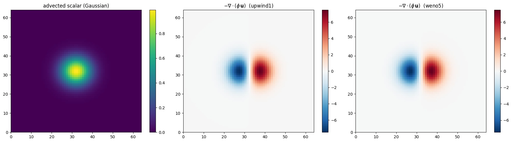
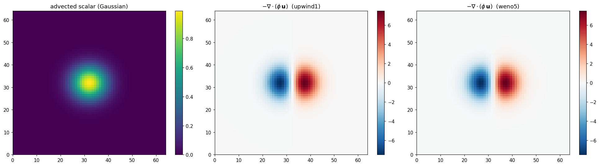
more sharply for the same grid. — Figure 2:The advective tendency $-\nabla\cdot(\phi\,\mathbf{u})$ of a Gaussian scalar under uniform rightward flow, computed with first-order upwind (centre) and fifth-order WENO (right). WENO resolves the leading and trailing edges far more sharply for the same grid.

From the Laplacian to elliptic inversion¶

The Laplacian diff.laplacian (a T → T map) is the building block of the elliptic problems the geophysical models solve at every step: recovering the streamfunction from vorticity, $\nabla^2\psi = \zeta$ , or the pressure from divergence. somax wraps these in dedicated spectral / multigrid solvers (the Helmholtz and Poisson solvers used by the QG and Navier–Stokes models), but they all rest on this discrete second-difference operator.

# Round-trip sanity: laplacian of sin/cos returns -8 pi^2 * psi analytically.
lap_psi = diff.laplacian(psi)
exact_lap = -8.0 * jnp.pi**2 * psi
rel_err = float(
    jnp.linalg.norm((lap_psi - exact_lap)[s]) / jnp.linalg.norm(exact_lap[s])
)
print(f"||laplacian(psi) - exact|| / ||exact|| (interior) = {rel_err:.3e}")

||laplacian(psi) - exact|| / ||exact|| (interior) = 3.129e-02

Summary¶

C-grid operators are stagger-changing: a derivative of a T-field lands on faces ((1)), a divergence of faces returns to centres ((2)).
Difference2D provides gradients, divergence, curl, and laplacian; Interpolation2D moves fields between positions (Table 1); Advection2D reconstructs fluxes with upwind or WENO schemes (Figure 2).
The discrete Laplacian underlies the elliptic solvers the QG and Navier–Stokes models invert each step.

The next chapter, boundary conditions, shows how the ghost halo carries the boundary data these operators read at the domain edge.

References¶

Durran, D. R. (2010). Numerical Methods for Fluid Dynamics: With Applications to Geophysics (2nd ed., Vol. 32). Springer. 10.1007/978-1-4419-6412-0
LeVeque, R. J. (2002). Finite Volume Methods for Hyperbolic Problems. Cambridge University Press. 10.1017/CBO9780511791253
Arakawa, A., & Lamb, V. R. (1977). Computational design of the basic dynamical processes of the UCLA general circulation model. Methods in Computational Physics, 17, 173–265.
Liu, X.-D., Osher, S., & Chan, T. (1994). Weighted essentially non-oscillatory schemes. Journal of Computational Physics, 115(1), 200–212. 10.1006/jcph.1994.1187
Shu, C.-W. (1998). Essentially non-oscillatory and weighted essentially non-oscillatory schemes for hyperbolic conservation laws. Advanced Numerical Approximation of Nonlinear Hyperbolic Equations, 1697, 325–432. 10.1007/BFb0096355