Boundary Conditions

The discrete operators of the previous chapter read one cell beyond each field point. At the edge of the domain that neighbour lies outside the physical region — it is a ghost cell, and what we write into it is the boundary condition. This chapter shows how finitevolX frames the interior with a ghost halo and how the standard boundary types — periodic, Dirichlet, Neumann, reflective, outflow — are each just a rule for filling those ghosts LeVeque (2002)Durran (2010).

What you will learn

How ghost cells turn a boundary condition into a local array update
The five canonical 1-D boundary types and their ghost-fill rules
How to compose per-face conditions with BoundaryConditionSet
The enforce_periodic shortcut somax models use most

Ghost cells: the boundary as an array update¶

Recall from the C-grid chapter that finitevolX stores an $n_x\times n_y$ interior inside an $(n_x{+}2)\times(n_y{+}2)$ array. The outermost ring is the ghost halo. A stencil at the first interior cell, say the $x$ -difference (1) reused here as

\big(\partial_x h\big)_{j,\,\frac12} \approx \frac{h_{j,1} - h_{j,0}}{\Delta x},

(1)

reads the ghost value $h_{j,0}$ . Choosing $h_{j,0}$ is choosing the boundary condition — no special-cased edge stencils are needed, which keeps the operators uniform across the whole grid. Each boundary type below is simply a different formula for the ghost value in terms of the interior.

The canonical boundary types¶

Table 1 lists the ghost-fill rules finitevolX implements as 1-D boundary objects. Let $\phi_{\text{int}}$ be the first interior value adjacent to the boundary and $\phi_{\text{ghost}}$ the ghost value to fill.

Table 1:Canonical boundary types and their ghost-fill rules. $\phi_{\text{int}}$ is the adjacent interior value; $h$ is the cell spacing normal to the boundary.

Type	finitevolX class	Ghost-fill rule	Physical meaning
Periodic	`Periodic1D`	$\phi_{\text{ghost}} = \phi_{\text{opposite interior}}$	domain wraps (channel, doubly-periodic box)
Dirichlet	`Dirichlet1D`	$\phi_{\text{ghost}} = 2c - \phi_{\text{int}}$	fixed boundary value $c$ (e.g. no-slip wall $u=0$ )
Neumann	`Neumann1D`	$\phi_{\text{ghost}} = \phi_{\text{int}} + g\,h$	fixed normal gradient $g$ (e.g. zero flux)
Reflective	`Reflective1D`	$\phi_{\text{ghost}} = -\phi_{\text{int}}$	mirror / free-slip symmetry
Outflow	`Outflow1D`	$\phi_{\text{ghost}} = \phi_{\text{int}}$	zero-gradient open boundary

The Dirichlet rule is worth a second look: setting the ghost to $2c-\phi_{\text{int}}$ makes the average of the ghost and interior cells equal $c$ , so the interpolated value at the boundary face is exactly the prescribed $c$ — the right way to impose a wall value on a cell-centred field.

import warnings

warnings.filterwarnings("ignore", message=r".*IProgress.*")

import importlib.util
from pathlib import Path

import finitevolx as fvx
import jax.numpy as jnp
import matplotlib.pyplot as plt

try:
    from IPython import get_ipython

    ipython = get_ipython()
except ImportError:
    ipython = None

if ipython is not None and importlib.util.find_spec("watermark") is not None:
    ipython.run_line_magic("load_ext", "watermark")
    ipython.run_line_magic("watermark", "-v -m -p numpy,jax,finitevolx,somax")
else:
    print("watermark extension not installed; skipping reproducibility readout.")

watermark extension not installed; skipping reproducibility readout.

Periodic boundaries: the `enforce_periodic` shortcut¶

Most somax models run on a doubly-periodic box and call the convenience enforce_periodic, which copies each interior edge into the opposite ghost ring. We can see it directly: fill the interior with a ramp, then check that the ghost row mirrors the opposite interior row.

grid = fvx.CartesianGrid2D.from_interior(nx_interior=16, ny_interior=16, Lx=1.0, Ly=1.0)
field = jnp.zeros((grid.Ny, grid.Nx))
ramp = jnp.arange(16 * 16, dtype=float).reshape(16, 16)
field = field.at[1:-1, 1:-1].set(ramp)

field_periodic = fvx.enforce_periodic(field)
# Ghost row 0 should equal the last interior row (-2) after wrapping.
wrapped = bool(jnp.allclose(field_periodic[0, 1:-1], field_periodic[-2, 1:-1]))
print(f"periodic wrap: ghost row 0 == interior row -2 ? {wrapped}")

periodic wrap: ghost row 0 == interior row -2 ? True

Composing per-face conditions with `BoundaryConditionSet`¶

Real basins mix conditions: a zonal channel is periodic east–west but walled north–south. BoundaryConditionSet assigns an independent 1-D condition to each of the four faces and applies them in one call. Here we build the channel configuration — periodic in $x$ , Dirichlet walls in $y$ .

channel_bc = fvx.BoundaryConditionSet(
    west=fvx.Periodic1D("west"),
    east=fvx.Periodic1D("east"),
    south=fvx.Dirichlet1D("south", value=0.0),
    north=fvx.Dirichlet1D("north", value=0.0),
)
field_channel = channel_bc(field, dx=grid.dx, dy=grid.dy)

# East-west wrap holds; north-south enforces the wall (face value 0).
ew_periodic = bool(jnp.allclose(field_channel[1:-1, 0], field_channel[1:-1, -2]))
south_face = field_channel[0, 1:-1] + field_channel[1, 1:-1]  # ghost + first interior
print(f"channel: east-west periodic ? {ew_periodic}")
print(
    f"channel: south wall face value ~ 0 ? {bool(jnp.allclose(south_face, 0.0, atol=1e-6))}"
)

channel: east-west periodic ? True
channel: south wall face value ~ 0 ? True

Visualising the boundary effect¶

Figure 1 contrasts the two configurations on the same interior field. Under fully periodic boundaries the ghost ring (outer frame) carries the wrapped opposite edge; under the channel configuration the north/south ghosts are the wall reflection while east/west still wrap.

IMG_DIR = Path.cwd().parent / "images" / "boundary_conditions"
IMG_DIR.mkdir(parents=True, exist_ok=True)

# A smoother interior field so the ghost ring is visually legible.
x = jnp.linspace(0.0, 1.0, grid.Nx)
y = jnp.linspace(0.0, 1.0, grid.Ny)
xx, yy = jnp.meshgrid(x, y)
smooth = jnp.zeros((grid.Ny, grid.Nx))
smooth = smooth.at[1:-1, 1:-1].set(
    (jnp.sin(3 * jnp.pi * xx) * jnp.sin(2 * jnp.pi * yy))[1:-1, 1:-1]
)

periodic_full = fvx.enforce_periodic(smooth)
channel_full = channel_bc(smooth, dx=grid.dx, dy=grid.dy)

fig, axes = plt.subplots(1, 3, figsize=(18, 5))
vlim = float(jnp.max(jnp.abs(smooth)))
kw = dict(cmap="RdBu_r", vmin=-vlim, vmax=vlim)
axes[0].pcolormesh(smooth, **kw)
axes[0].set(title="interior field (ghosts = 0)")
axes[1].pcolormesh(periodic_full, **kw)
axes[1].set(title="periodic ghosts (enforce_periodic)")
axes[2].pcolormesh(channel_full, **kw)
axes[2].set(title="channel: periodic x, wall y")
for ax in axes:
    # mark the interior/ghost boundary
    ax.axhline(1, color="k", lw=0.6)
    ax.axhline(grid.Ny - 1, color="k", lw=0.6)
    ax.axvline(1, color="k", lw=0.6)
    ax.axvline(grid.Nx - 1, color="k", lw=0.6)
fig.tight_layout()
fig.savefig(IMG_DIR / "bc_comparison.png", dpi=110, bbox_inches="tight")
plt.show()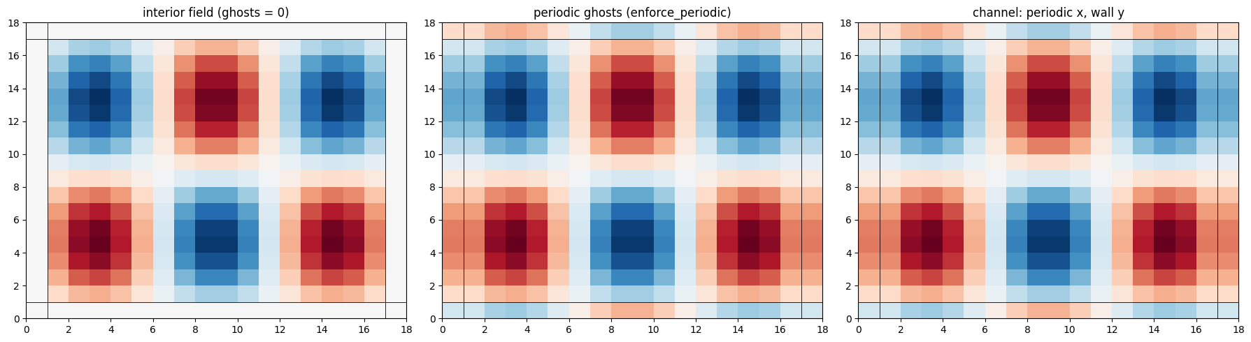

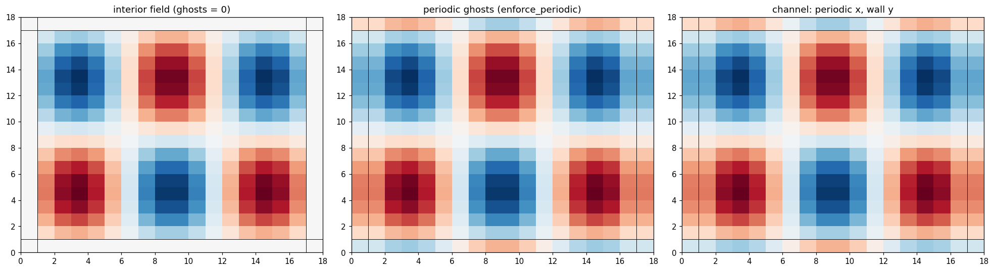
The same interior field (left, ghosts zeroed) with periodic ghosts filled by
enforce_periodic (centre) and with the channel BoundaryConditionSet
(right; periodic in x, Dirichlet walls in y). The thin black frame marks
the interior/ghost boundary. — Figure 1:The same interior field (left, ghosts zeroed) with periodic ghosts filled by `enforce_periodic` (centre) and with the channel `BoundaryConditionSet` (right; periodic in $x$ , Dirichlet walls in $y$ ). The thin black frame marks the interior/ghost boundary.

How somax models use boundary conditions¶

Each somax model implements apply_boundary_conditions(state), which the time integrator calls before every right-hand-side evaluation so the operators always read boundary-consistent ghosts. A doubly-periodic model maps enforce_periodic over each state field; a walled model applies the appropriate wall (Dirichlet / reflective) condition per field and face. The boundary type is therefore part of the model’s physical specification, not an afterthought — it is enforced at every step, never skipped.

Summary¶

A boundary condition is a rule for filling the ghost cells the stencils read ((1)); no special edge stencils are required.
The five canonical types — periodic, Dirichlet, Neumann, reflective, outflow — are distinct ghost-fill formulas (Table 1).
enforce_periodic handles the common doubly-periodic case; BoundaryConditionSet composes independent per-face conditions (Figure 1).
somax models enforce their boundary conditions inside apply_boundary_conditions, called before every RHS evaluation.

This completes the Phase 0 foundations — grids, operators, and boundary conditions. The model chapters build on these primitives to assemble the shallow-water and quasi-geostrophic dynamics.

References¶

LeVeque, R. J. (2002). Finite Volume Methods for Hyperbolic Problems. Cambridge University Press. 10.1017/CBO9780511791253
Durran, D. R. (2010). Numerical Methods for Fluid Dynamics: With Applications to Geophysics (2nd ed., Vol. 32). Springer. 10.1007/978-1-4419-6412-0