Composing finitevolX with pipekit
finitevolX ships two tiers of the same operators:
Tier A  finitevolx                 Difference2D(grid).diff_x_T_to_U(h)
        arrays in, arrays out      eqx.Module / pure function, no config
                │
                ▼
Tier B  finitevolx.pipekit         Difference(grid=G, axis="x", src="T", dst="U")
        pipekit Operators          JSON config · eqx leaves · Sequential / Graph
                │
                ▼
pipekit Graph / Sequential / Rollout — diagnostics pipelines, DA glue, emulators
Tier B is the same arithmetic (each operator is one Tier-A call) with a
configuration you can save, a node you can wire into a pipekit_ops.Graph,
and pytree leaves (f₀, β, g′, Δt) that jax.grad reaches.
When to use which. A model's right-hand side belongs in your model
code — in somax, a Term tree, which is already pytree-native and
IMEX-partitionable. Tier B is for everything around the model:
diagnostics over a trajectory, stagger moves for plotting, ghost-ring and
mask handling, reductions, and observation operators for assimilation.
Below we still build a model RHS as a graph, because it makes a compact,
checkable example.
Install the extra: pip install "finitevolx[pipekit]". Theory of the
operators: C-grid discretization.
from pathlib import Path
import json
import time

import equinox as eqx
import jax
import jax.numpy as jnp
import matplotlib

matplotlib.use("Agg")
import matplotlib.pyplot as plt
from pipekit_ops import Graph, Input, Operator
from pipekit_jax import Rollout

import finitevolx as fvx
from finitevolx import pipekit as fp

jax.config.update("jax_enable_x64", True)

IMG_DIR = Path(__file__).resolve().parent.parent / "images" / "pipekit_composition"
IMG_DIR.mkdir(parents=True, exist_ok=True)
1. Linear rotating shallow water as a graph
On a doubly periodic C-grid with mean depth $H$, gravity $g$ and an $f$-plane $f = f_0$, for thickness anomaly $h$ (T-points) and velocity $(u, v)$ (U- and V-points):
$$ \partial_t h = -H\,(\delta_x u + \delta_y v), \qquad \partial_t u = +f\,\bar v - g\,\delta_x h, \qquad \partial_t v = -f\,\bar u - g\,\delta_y h . $$
The energy $E = \tfrac12 \sum (H(u^2 + v^2) + g h^2)\,\Delta A$ is
conserved by the spatial scheme. A grid is a static tuple
(nx_interior, ny_interior, Lx, Ly).
N = 128
G_SPEC = (N, N, 1.0, 1.0)
H, GRAV, F0 = 1.0, 1.0, 20.0
DT = 0.25 / N  # CFL  c Δt / Δx = 0.25,  c = √(gH) = 1


def sw_tendency(f0: float = F0) -> Graph:
    h, u, v = Input("h"), Input("u"), Input("v")
    # ghost ring, periodic                                   [*, Ny, Nx] each
    hp, up, vp = (fp.FillGhosts(kind="periodic")(x) for x in (h, u, v))
    # ∂ₜh = −H ∇·(u, v)                                       T
    dh = fp.LinComb(coeffs=(-H,))(fp.Divergence(grid=G_SPEC)(up, vp))
    # (+f v̄, −f ū)                                           (U, V)
    cor = fp.Coriolis(grid=G_SPEC, f0=f0)(up, vp)
    # δₓh, δᵧh                                                U, V
    gx = fp.Difference(grid=G_SPEC, axis="x", src="T", dst="U")(hp)
    gy = fp.Difference(grid=G_SPEC, axis="y", src="T", dst="V")(hp)
    # ∂ₜu = f v̄ − g δₓh,   ∂ₜv = −f ū − g δᵧh
    du = fp.LinComb(coeffs=(1.0, -GRAV))(fp.Pick(index=0)(cor), gx)
    dv = fp.LinComb(coeffs=(1.0, -GRAV))(fp.Pick(index=1)(cor), gy)
    return Graph(inputs={"h": h, "u": u, "v": v}, outputs={"h": dh, "u": du, "v": dv})


rhs = sw_tendency()
print(rhs.describe())
A step is ExplicitStep (finitevolX's rk4_step over the graph), and a
trajectory is pipekit_jax.Rollout: one jax.lax.scan, so compile time
does not grow with the number of steps.
grid = fp.build_grid(G_SPEC)
y = (jnp.arange(grid.Ny) - 0.5) / N
x = (jnp.arange(grid.Nx) - 0.5) / N
Y, X = jnp.meshgrid(y, x, indexing="ij")
h0 = 0.1 * jnp.exp(-((X - 0.5) ** 2 + (Y - 0.5) ** 2) / (2 * 0.05**2))
s0 = {"h": h0, "u": jnp.zeros_like(h0), "v": jnp.zeros_like(h0)}

N_STEPS, SAVE = 400, 40
step = fp.ExplicitStep(rhs=rhs, dt=DT)
model = Rollout(step=step, n_steps=N_STEPS, save_every=SAVE)
run = eqx.filter_jit(lambda m, s: m(s))

t = time.perf_counter()
traj = jax.block_until_ready(run(model, s0))  # {h, u, v: [11, Ny, Nx]}
print(f"compile + run: {time.perf_counter() - t:.1f} s;  h: {traj['h'].shape}")
Same program as hand-written finitevolX
The same step written directly against Tier A gives a bit-identical
state and compiles to the same program up to a few fusions (104 vs 101
here, on CPU), with no gathers or scatters on either side: under jit
the pipekit layer is free.
D = fvx.Difference2D(grid=grid)
f_T = F0 * jnp.ones((grid.Ny, grid.Nx))


def rhs_tier_a(s):
    h, u, v = (fvx.enforce_periodic(s[k]) for k in "huv")
    cu, cv = fvx.Coriolis2D(grid=grid)(u, v, f_T)
    return {
        "h": -H * D.divergence(u, v),
        "u": cu - GRAV * D.diff_x_T_to_U(h),
        "v": cv - GRAV * D.diff_y_T_to_V(h),
    }


def step_tier_a(s):
    return fvx.rk4_step(s, rhs_tier_a, DT)


step_jit = jax.jit(step_tier_a)
dyn, static = eqx.partition(step, eqx.is_array)
step_pk = jax.jit(lambda d, s: eqx.combine(d, static)(s))
hlo_pk = step_pk.lower(dyn, s0).compile().as_text()
hlo_a = step_jit.lower(s0).compile().as_text()


def count(text):
    return {k: text.count(f" {k}(") for k in ("fusion", "gather", "scatter")}


diff = max(float(jnp.abs(step_pk(dyn, s0)[k] - step_jit(s0)[k]).max()) for k in "huv")
print("pipekit step :", count(hlo_pk))
print("Tier-A step  :", count(hlo_a))
print("max |Δ| after one step:", diff)
2. A diagnostics pipeline over the trajectory
Every Tier-B operator takes [*batch, Ny, Nx], so one graph evaluates
relative vorticity ζ (X-points), the Okubo–Weiss parameter $W$
(T-points) and the total energy $E$ for every saved time at once; the
reductions keep the time axis, [T, Ny, Nx] → [T].
h, u, v = Input("h"), Input("u"), Input("v")
hp, up, vp = (fp.FillGhosts(kind="periodic")(x) for x in (h, u, v))
ke = fp.LinComb(coeffs=(H,))(fp.KineticEnergy(grid=G_SPEC)(up, vp))
ape = fp.AvailablePE(grid=G_SPEC, g_prime=GRAV)(hp)
diagnostics = Graph(
    inputs={"h": h, "u": u, "v": v},
    outputs={
        "zeta": fp.RelativeVorticity(grid=G_SPEC)(up, vp),
        "OW": fp.OkuboWeiss(grid=G_SPEC)(up, vp),
        "E": fp.TotalEnergy(grid=G_SPEC)(ke, ape),
    },
)
diag = eqx.filter_jit(lambda g, t: g(**t))(diagnostics, traj)
drift = jnp.abs(diag["E"] / diag["E"][0] - 1)
print({k: v.shape for k, v in diag.items()})
print(f"max |E/E₀ − 1| over {N_STEPS} steps: {float(drift.max()):.1e}")
times = jnp.arange(traj["h"].shape[0]) * SAVE * DT
fig, axes = plt.subplots(1, 4, figsize=(16, 3.6))
inner = (slice(1, -1), slice(1, -1))
for ax, (field, title, cmap) in zip(
    axes[:3],
    [
        (traj["h"][-1][inner], f"h at t = {float(times[-1]):.2f}", "RdBu_r"),
        (diag["zeta"][-1][inner], "relative vorticity ζ", "PuOr_r"),
        (diag["OW"][-1][inner], "Okubo–Weiss W", "PiYG"),
    ],
    strict=True,
):
    lim = float(jnp.abs(field).max())
    im = ax.imshow(field, origin="lower", cmap=cmap, vmin=-lim, vmax=lim)
    ax.set_title(title)
    ax.set_xticks([])
    ax.set_yticks([])
    fig.colorbar(im, ax=ax, shrink=0.8)
axes[3].semilogy(times[1:], drift[1:], "o-")
axes[3].set_xlabel("t")
axes[3].set_title("|E(t)/E(0) − 1|")
fig.tight_layout()
fig.savefig(IMG_DIR / "diagnostics.png", dpi=110, bbox_inches="tight")
plt.show()
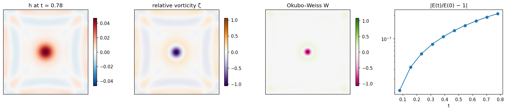
The energy drift is RK4 time error alone: halving Δt divides it by about
32 (see tests/test_pipekit_diagnostics.py).
3. Gradients through the graph
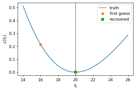
f₀ is a leaf of the Coriolis node, so jax.grad of a loss on the
trajectory reaches it through Rollout, ExplicitStep and the graph.
Twin experiment: observe $h$ from the run with $f_0 = 20$, start from a
wrong guess, and look at the misfit
$\mathcal{L}(f_0) = \sum_t \lVert h_t(f_0) - h_t^{\text{obs}} \rVert^2$.
short = 100
obs = run(Rollout(step=step, n_steps=short, save_every=20), s0)["h"]


def misfit(f0):
    stp = fp.ExplicitStep(rhs=sw_tendency(f0), dt=DT)
    pred = Rollout(step=stp, n_steps=short, save_every=20)(s0)["h"]
    return jnp.sum((pred - obs) ** 2)


misfit_jit = jax.jit(misfit)
grad_jit = jax.jit(jax.grad(misfit))
f0_grid = jnp.linspace(14.0, 26.0, 25)
losses = jnp.stack([misfit_jit(f) for f in f0_grid])

f0_guess, eps = 16.0, 1e-3
g_ad = float(grad_jit(f0_guess))
g_fd = float((misfit_jit(f0_guess + eps) - misfit_jit(f0_guess - eps)) / (2 * eps))
print(f"dL/df0 at f0 = {f0_guess}: autodiff {g_ad:.6e}, finite difference {g_fd:.6e}")

# a few Newton-like steps on the secant of the gradient recover f0
f_a, f_b = 16.0, 17.0
for _ in range(6):
    g_a, g_b = float(grad_jit(f_a)), float(grad_jit(f_b))
    f_a, f_b = f_b, f_b - g_b * (f_b - f_a) / (g_b - g_a)
print(f"recovered f0 = {f_b:.6f} (truth {F0})")
fig, ax = plt.subplots(figsize=(5, 3.4))
ax.plot(f0_grid, losses, "-")
ax.axvline(F0, color="k", ls="--", lw=1, label="truth")
ax.plot([f0_guess], [misfit_jit(f0_guess)], "o", label="first guess")
ax.plot([f_b], [misfit_jit(f_b)], "s", label="recovered")
ax.set_xlabel("$f_0$")
ax.set_ylabel(r"$\mathcal{L}(f_0)$")
ax.legend()
fig.tight_layout()
fig.savefig(IMG_DIR / "misfit.png", dpi=110, bbox_inches="tight")
plt.show()
4. Configuration round trip
Every operator's state is plain JSON; Operator.from_state rebuilds
it. The grid is a tuple, learnable values are numbers.
op = fp.Coriolis(grid=G_SPEC, f0=F0, beta=0.0)
record = json.dumps(op.state)
print(record)
same = Operator.from_state(json.loads(record))
print(type(same).__name__, same.grid, float(same.f0))
ApplyMask holds a Mask2D and ExplicitStep holds a whole graph, so
their records are for inspection only: ApplyMask is forbid_in_yaml
and persists through serialize_weights / with_weights, and nested
graphs are rebuilt by pipekit's YAML loader rather than from_state.