SPDE Priors on the C-Grid with gaussx¶

A data-assimilation background covariance $B$ (or a Gaussian-process prior for an emulator) should live on the model's own grid and respect its coastline: two points on either side of a peninsula are far apart for the ocean even when they are close in a straight line. The SPDE approach (Lindgren, Rue & Lindström, 2011) gets this for free. Let

$\psi$ be a field on the ψ-points of the C-grid,
$\nabla^2_h$ the model's 5-point Laplacian, with the land mask applied as $\psi = 0$ on land,
$\kappa > 0$ an inverse correlation length ($\ell \approx \sqrt{8\nu}/\kappa$),
$\alpha \in \{1, 2, \dots\}$ the smoothness order and $\tau$ an amplitude.

The Matérn-type precision is

$$ Q = \tau^2\,(\kappa^2 - \nabla^2_h)^{\alpha}, \qquad B = Q^{-1}. $$

finitevolX exposes $\nabla^2_h - \lambda$ as a structured gaussx operator, so $Q$ inherits gaussx's exact solve, log-determinant and square root without ever forming a matrix. The marginal variance $\operatorname{diag}(Q^{-1})$ is the exception: gaussx.diag_inv builds the dense $(N_y N_x)^2$ basis for this operator (about 1.2 GB at $96 \times 128$), so section 1 computes it from the two 1-D bases instead.

helmholtz_operator(shape, dx, dy, lambda_, bc) — the rectangle operator as a gaussx.DiagonalizedOperator (FFT / DST-I / DCT-II);
masked_helmholtz_operator(mask, dx, dy, lambda_) — the masked operator of masked_laplacian as a gaussx.MaskedOperator whose solve is the capacitance method.

On a uniform grid the lumped mass matrix of the SPDE is $h^2 I$; it is absorbed into $\tau$ here.

In [ ]:

Copied!





from pathlib import Path

import gaussx
import jax
import jax.numpy as jnp
import matplotlib

matplotlib.use("Agg")
import matplotlib.pyplot as plt
import numpy as np

import finitevolx as fvx

jax.config.update("jax_enable_x64", True)

IMG_DIR = Path(__file__).resolve().parent.parent / "images" / "spde_prior"
IMG_DIR.mkdir(parents=True, exist_ok=True)
from pathlib import Path

import gaussx
import jax
import jax.numpy as jnp
import matplotlib

matplotlib.use("Agg")
import matplotlib.pyplot as plt
import numpy as np

import finitevolx as fvx

jax.config.update("jax_enable_x64", True)

IMG_DIR = Path(__file__).resolve().parent.parent / "images" / "spde_prior"
IMG_DIR.mkdir(parents=True, exist_ok=True)

1. Rectangle: exact samples and marginal variance¶

On a rectangle with Neumann walls (DCT-II), $K = \kappa^2 - \nabla^2_h$ is diagonal in the DCT basis with eigenvalues $\kappa^2 - \Lambda_{ji}$, so $Q = \tau^2 K^\alpha$ is too. A sample is $x = Q^{-1/2} z$ with $z \sim \mathcal N(0, I)$, and $\operatorname{diag}(Q^{-1})$ is exact.

In [ ]:

Copied!





ny, nx = 96, 128  # [Ny, Nx]
Lx, Ly = 2.0, 1.5
dx, dy = Lx / nx, Ly / ny
ell = 0.15  # correlation length
alpha = 2
kappa = np.sqrt(8 * (alpha - 1)) / ell  # ν = α − d/2 = 1 in 2-D
tau = 1.0

# K = κ² − ∇²_h = −(∇²_h − κ²), a DiagonalizedOperator, never materialised
K = -fvx.helmholtz_operator((ny, nx), dx, dy, lambda_=kappa**2, bc="dct")
# Q = τ² K^α: same transform pair, eigenvalues τ² (κ² − Λ)^α
Q = gaussx.DiagonalizedOperator(
    tau**2 * K.eigenvalues**alpha, K.forward, K.inverse, K.in_shape, normal=True
)


def marginal_variance(Q: gaussx.DiagonalizedOperator) -> jnp.ndarray:
    """diag(Q⁻¹) for a separable orthonormal basis V = Vy ⊗ Vx.

    diag(Vᵀ Λ⁻¹ V)[j, i] = Σ_{k,l} Vy[k, j]² Vx[l, i]² / Λ[k, l], computed
    from the two 1-D bases (O(Ny² + Nx²) memory) rather than the
    (Ny·Nx)² matrix.
    """
    ny, nx = Q.in_shape
    # 1-D orthonormal DCT-II matrices: column j is the transform of e_j
    Vy = fvx.dctn(jnp.eye(ny), type=2, axes=[0], norm="ortho")  # [k, j]
    Vx = fvx.dctn(jnp.eye(nx), type=2, axes=[0], norm="ortho")  # [l, i]
    return (Vy**2).T @ (1.0 / Q.eigenvalues) @ (Vx**2)  # [Ny, Nx]


# rescale τ so the interior marginal standard deviation is 1
var = marginal_variance(Q)  # [Ny, Nx]
tau = float(jnp.sqrt(var[ny // 2, nx // 2]))
Q = gaussx.DiagonalizedOperator(
    tau**2 * K.eigenvalues**alpha, K.forward, K.inverse, K.in_shape, normal=True
)
std = jnp.sqrt(marginal_variance(Q))  # [Ny, Nx]

# exact samples x = Q^{-1/2} z, elementwise in the eigenvalues
B_half = gaussx.sqrt(gaussx.inv(Q))
keys = jax.random.split(jax.random.PRNGKey(0), 2)
samples = [
    B_half.mv(jax.random.normal(k, (ny * nx,))).reshape(ny, nx) for k in keys
]
print(f"logdet Q = {float(gaussx.logdet(Q)):.1f}")
ny, nx = 96, 128  # [Ny, Nx]
Lx, Ly = 2.0, 1.5
dx, dy = Lx / nx, Ly / ny
ell = 0.15  # correlation length
alpha = 2
kappa = np.sqrt(8 * (alpha - 1)) / ell  # ν = α − d/2 = 1 in 2-D
tau = 1.0

# K = κ² − ∇²_h = −(∇²_h − κ²), a DiagonalizedOperator, never materialised
K = -fvx.helmholtz_operator((ny, nx), dx, dy, lambda_=kappa**2, bc="dct")
# Q = τ² K^α: same transform pair, eigenvalues τ² (κ² − Λ)^α
Q = gaussx.DiagonalizedOperator(
    tau**2 * K.eigenvalues**alpha, K.forward, K.inverse, K.in_shape, normal=True
)


def marginal_variance(Q: gaussx.DiagonalizedOperator) -> jnp.ndarray:
    """diag(Q⁻¹) for a separable orthonormal basis V = Vy ⊗ Vx.

    diag(Vᵀ Λ⁻¹ V)[j, i] = Σ_{k,l} Vy[k, j]² Vx[l, i]² / Λ[k, l], computed
    from the two 1-D bases (O(Ny² + Nx²) memory) rather than the
    (Ny·Nx)² matrix.
    """
    ny, nx = Q.in_shape
    # 1-D orthonormal DCT-II matrices: column j is the transform of e_j
    Vy = fvx.dctn(jnp.eye(ny), type=2, axes=[0], norm="ortho")  # [k, j]
    Vx = fvx.dctn(jnp.eye(nx), type=2, axes=[0], norm="ortho")  # [l, i]
    return (Vy**2).T @ (1.0 / Q.eigenvalues) @ (Vx**2)  # [Ny, Nx]


# rescale τ so the interior marginal standard deviation is 1
var = marginal_variance(Q)  # [Ny, Nx]
tau = float(jnp.sqrt(var[ny // 2, nx // 2]))
Q = gaussx.DiagonalizedOperator(
    tau**2 * K.eigenvalues**alpha, K.forward, K.inverse, K.in_shape, normal=True
)
std = jnp.sqrt(marginal_variance(Q))  # [Ny, Nx]

# exact samples x = Q^{-1/2} z, elementwise in the eigenvalues
B_half = gaussx.sqrt(gaussx.inv(Q))
keys = jax.random.split(jax.random.PRNGKey(0), 2)
samples = [
    B_half.mv(jax.random.normal(k, (ny * nx,))).reshape(ny, nx) for k in keys
]
print(f"logdet Q = {float(gaussx.logdet(Q)):.1f}")

In [ ]:

Copied!





fig, axes = plt.subplots(1, 3, figsize=(15, 4))
extent = [0, Lx, 0, Ly]
for ax, s, title in zip(axes[:2], samples, ["sample 1", "sample 2"]):
    im = ax.imshow(np.asarray(s), origin="lower", cmap="RdBu_r", extent=extent)
    ax.set_title(title)
    fig.colorbar(im, ax=ax, shrink=0.8)
im = axes[2].imshow(np.asarray(std), origin="lower", cmap="viridis", extent=extent)
axes[2].set_title("marginal std $\\sqrt{\\mathrm{diag}(Q^{-1})}$")
fig.colorbar(im, ax=axes[2], shrink=0.8)
fig.tight_layout()
fig.savefig(IMG_DIR / "rectangle_samples.png", dpi=120, bbox_inches="tight")
plt.show()
fig, axes = plt.subplots(1, 3, figsize=(15, 4))
extent = [0, Lx, 0, Ly]
for ax, s, title in zip(axes[:2], samples, ["sample 1", "sample 2"]):
    im = ax.imshow(np.asarray(s), origin="lower", cmap="RdBu_r", extent=extent)
    ax.set_title(title)
    fig.colorbar(im, ax=ax, shrink=0.8)
im = axes[2].imshow(np.asarray(std), origin="lower", cmap="viridis", extent=extent)
axes[2].set_title("marginal std $\\sqrt{\\mathrm{diag}(Q^{-1})}$")
fig.colorbar(im, ax=axes[2], shrink=0.8)
fig.tight_layout()
fig.savefig(IMG_DIR / "rectangle_samples.png", dpi=120, bbox_inches="tight")
plt.show()

Exact Matérn samples and marginal standard deviation

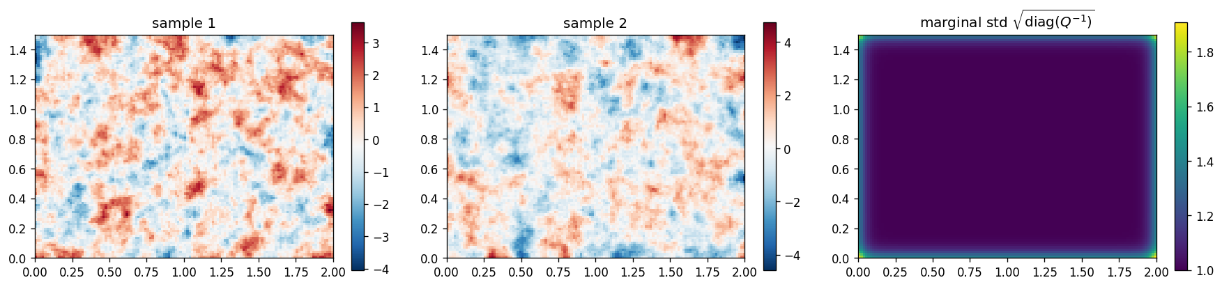
The Neumann walls inflate the variance within about one correlation length of the boundary (up to $2\times$ on an edge, $4\times$ in a corner); extend the domain beyond the region of interest when that matters.

2. A basin with a peninsula: correlations follow the ocean¶

With a land mask, $K_m = \kappa^2 - \nabla^2_h$ restricted to the wet points is no longer diagonal in any fast basin, but masked_helmholtz_operator solves it exactly with the capacitance method (two DST solves per right-hand side, after a one-off factorisation over the coastal ring). For $\alpha = 2$,

$$ B\,v = \tau^{-2} K_m^{-1} K_m^{-1} v, $$

so one column of $B$ (the correlation with a single point) costs two solves. Compare it with the same prior on the rectangle, which ignores the land.

In [ ]:

Copied!





ny, nx = 96, 96
L = 1.5
dx = dy = L / nx
wet = np.zeros((ny, nx), dtype=bool)
wet[3:-3, 3:-3] = True  # basin with closed walls
wet[3:62, 44:52] = False  # a peninsula from the south wall
wet_flat = wet.ravel()

K_m = -fvx.masked_helmholtz_operator(wet, dx, dy, lambda_=kappa**2)
K_rect = -fvx.helmholtz_operator((ny, nx), dx, dy, lambda_=kappa**2, bc="dct")


def b_column_masked(j: int, i: int) -> np.ndarray:
    """Row (j, i) of B = K_m^{-2}, on the full grid with land set to NaN."""
    v = jnp.zeros(ny * nx).at[j * nx + i].set(1.0)[wet_flat]  # [n_wet]
    col = gaussx.solve(K_m, gaussx.solve(K_m, v))  # [n_wet]
    full = np.full(ny * nx, np.nan)
    full[wet_flat] = np.asarray(col)
    full = full.reshape(ny, nx)
    return full / full[j, i]


def b_column_rect(j: int, i: int) -> np.ndarray:
    """Row (j, i) of the rectangle prior, which ignores the land."""
    v = jnp.zeros(ny * nx).at[j * nx + i].set(1.0)
    col = gaussx.solve(K_rect, gaussx.solve(K_rect, v)).reshape(ny, nx)
    col = np.asarray(col / col[j, i])
    return np.where(wet, col, np.nan)


point = (30, 42)  # just west of the peninsula
corr_masked = b_column_masked(*point)
corr_rect = b_column_rect(*point)
east = (30, 53)  # just east of it, 11 cells (0.17) away
print(
    f"correlation across the peninsula: masked {corr_masked[east]:.2e}, "
    f"rectangle {corr_rect[east]:.3f}"
)
ny, nx = 96, 96
L = 1.5
dx = dy = L / nx
wet = np.zeros((ny, nx), dtype=bool)
wet[3:-3, 3:-3] = True  # basin with closed walls
wet[3:62, 44:52] = False  # a peninsula from the south wall
wet_flat = wet.ravel()

K_m = -fvx.masked_helmholtz_operator(wet, dx, dy, lambda_=kappa**2)
K_rect = -fvx.helmholtz_operator((ny, nx), dx, dy, lambda_=kappa**2, bc="dct")


def b_column_masked(j: int, i: int) -> np.ndarray:
    """Row (j, i) of B = K_m^{-2}, on the full grid with land set to NaN."""
    v = jnp.zeros(ny * nx).at[j * nx + i].set(1.0)[wet_flat]  # [n_wet]
    col = gaussx.solve(K_m, gaussx.solve(K_m, v))  # [n_wet]
    full = np.full(ny * nx, np.nan)
    full[wet_flat] = np.asarray(col)
    full = full.reshape(ny, nx)
    return full / full[j, i]


def b_column_rect(j: int, i: int) -> np.ndarray:
    """Row (j, i) of the rectangle prior, which ignores the land."""
    v = jnp.zeros(ny * nx).at[j * nx + i].set(1.0)
    col = gaussx.solve(K_rect, gaussx.solve(K_rect, v)).reshape(ny, nx)
    col = np.asarray(col / col[j, i])
    return np.where(wet, col, np.nan)


point = (30, 42)  # just west of the peninsula
corr_masked = b_column_masked(*point)
corr_rect = b_column_rect(*point)
east = (30, 53)  # just east of it, 11 cells (0.17) away
print(
    f"correlation across the peninsula: masked {corr_masked[east]:.2e}, "
    f"rectangle {corr_rect[east]:.3f}"
)

In [ ]:

Copied!





fig, axes = plt.subplots(1, 2, figsize=(12, 5))
for ax, corr, title in zip(
    axes,
    [corr_rect, corr_masked],
    ["rectangle prior (ignores land)", "masked prior (SPDE on the basin)"],
):
    land = np.where(wet, np.nan, 1.0)
    ax.imshow(land, origin="lower", cmap="Greys", vmin=0, vmax=1.5, extent=[0, L, 0, L])
    im = ax.imshow(corr, origin="lower", cmap="magma", vmin=0, vmax=1, extent=[0, L, 0, L])
    ax.plot((point[1] + 0.5) * dx, (point[0] + 0.5) * dy, "c*", ms=12)
    ax.set_title(title)
    fig.colorbar(im, ax=ax, shrink=0.8, label="correlation with ★")
fig.tight_layout()
fig.savefig(IMG_DIR / "peninsula_correlation.png", dpi=120, bbox_inches="tight")
plt.show()
fig, axes = plt.subplots(1, 2, figsize=(12, 5))
for ax, corr, title in zip(
    axes,
    [corr_rect, corr_masked],
    ["rectangle prior (ignores land)", "masked prior (SPDE on the basin)"],
):
    land = np.where(wet, np.nan, 1.0)
    ax.imshow(land, origin="lower", cmap="Greys", vmin=0, vmax=1.5, extent=[0, L, 0, L])
    im = ax.imshow(corr, origin="lower", cmap="magma", vmin=0, vmax=1, extent=[0, L, 0, L])
    ax.plot((point[1] + 0.5) * dx, (point[0] + 0.5) * dy, "c*", ms=12)
    ax.set_title(title)
    fig.colorbar(im, ax=ax, shrink=0.8, label="correlation with ★")
fig.tight_layout()
fig.savefig(IMG_DIR / "peninsula_correlation.png", dpi=120, bbox_inches="tight")
plt.show()

Correlation with one point, rectangle vs masked prior

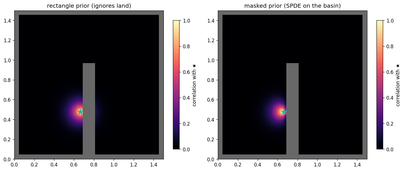
The rectangle prior correlates the two sides of the peninsula through the land; the masked prior has to go around it, so the correlation across is much weaker. The same operator gives $\log\det Q$ (for hyperparameter likelihoods) through gaussx.logdet, and is differentiable in $\kappa$ and $\tau$ for learning them.

Where to go next¶

Use $B$ as the background covariance in an EnKF / 3D-Var update with gaussx's Kalman primitives.
Swap $\nabla^2_h$ for an anisotropic or variable-coefficient operator (e.g. MultigridSolver with face coefficients) and solve with gaussx.CGSolver(preconditioner=fvx.make_gaussx_multigrid_preconditioner(mg)).