gridax: analysis grids for JAX
gridax is the stack’s library for the geometry of the grids data arrive on: rectilinear lon/lat grids, curvilinear and swath grids, their cell corners, areas and metrics on the sphere or the ellipsoid, vertical coordinates and the remapping between them, and the finite differences used to analyse a field on them. Its grids carry no CRS; geoarray attaches one. It does not own the grids a model steps on: finitevolX’s C-grids and spectraldiffx’s spectral grids are those libraries’ discretisations and stay with them. It sits at GeoNumerics tier 1, on geophysix and functax. Status: proposed, at design-sketch depth; revised on 5 Nov 2026 after reading finitevolX 0.1.0 and spectraldiffx.
At a glance
| Layer, tier | GeoNumerics, tier 1 |
| Imports | geophysix, functax; JAX, NumPy, Equinox |
| Imported by | diagnostix, tracerax; geoarray, geoops, xrops |
| Takes over | the finite-difference engine of geoops geom (difference, difference_offsets, difference_coeffs, nonuniform_coeffs) and the calculus built on it; the partials and grid_metrics_from_coords of xrops grad; xrops’ vertical remap kernels; the geometry behind geoarray’s SwathGrid and CurvilinearGrid labels |
| Does not own | model grids, their masks and vertical modes (finitevolX); spectral grids, transforms and their nodes (spectraldiffx); affine grids, point location and interpolation (functax); the CRS and the data (geoarray) |
| Status | proposed; no repository yet |
| Tracked in | the layer map; the companion geophysix and functax designs |
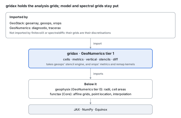
Where gridax sits · geonumerics tier 1.
gridax sits one tier above geophysix, whose radii and cell areas it uses, and imports functax for affine grids and interpolation. The libraries that analyse fields (diagnostix, tracerax’s binning) and the carriers (geoarray, geoops, xrops) import it; the libraries that step a model on their own grids do not need it. This page is the design; core types, algorithms and the code survey are in gridax: design details.
The problem
The methane example meets four kinds of grid before it reaches an emission rate: the instrument’s swath, the reanalysis’ model levels, the lon/lat grid the result is mapped on, and the staggered box the plume is transported in. The first three are where observations and products sit; the fourth is where a model steps. Only the first three are gridax’s question:
| Step | The grid fact it needs | Where it is coded today |
|---|---|---|
| Pixel areas of a scene in sensor geometry | the corners and areas of swath cells | not yet: geoarray’s SwathGrid labels the row col dims and holds the CRS; lat/lon are leaves on the carrier, and nothing computes corners or areas |
| Wind at plume height from model levels | a vertical coordinate, remapped onto height | xrops remap_axis and remap_axis_columns, with the ToHeight, ToPressureLevels, ToSigma and ToIsopycnal presets; xrops hypsometric_height |
| Spacings and areas of a lon/lat product | face lengths and cell areas on the sphere or the ellipsoid | xrops grid_metrics_from_coords; geoops pixel_area, the determinant of the affine transform, right only on a projected grid |
| Flux divergence and wind shear on a product | finite differences on an analysis grid, often non-uniform and with gaps | geoops geom: the stencil engine (difference, nonuniform_coeffs) and Gradient2D, Divergence2D, Curl2D, Laplacian2D with their 1-D and 3-D forms; xrops grad, which delegates every stencil to geoops.geom.difference |
| Plume transport in a box | a staggered C-grid with a ghost ring, masks and boundary conditions | finitevolX CartesianGrid3D with Mask3D, wrapped by plumax PlumeGrid3D, and that is where it stays |
The duplication is on the analysis side. Metrics are computed in xrops and approximated in geoops, and the only finite-difference engine for analysis grids lives in geoops, so xrops imports the GeoArray toolkit to differentiate an xarray field. The model side is not duplicated: finitevolX’s grids are read by 22 of its own modules and built directly by every model on top of it, and spectraldiffx’s grids are its transforms. An earlier draft of this tab proposed moving both here; the code says otherwise (decisions 3 and 4).
Three kinds of grid, and gridax’s one
The stack has three kinds of grid that look alike and are not:
| Kind | What defines it | Who owns it | Today |
|---|---|---|---|
| Model grid | the discretisation a model steps on: a staggering its schemes assume, a ghost ring for boundary conditions, uniform spacings, masks that say which stencils fit | finitevolX | ArakawaCGrid*, CartesianGrid*, SphericalGrid2D/3D, CylindricalGrid*, Mask1D/2D/3D |
| Spectral grid | the nodes of a transform: wavenumbers and a dealiasing rule, Gauss–Legendre or Chebyshev nodes with their weights, Legendre tables and differentiation matrices | spectraldiffx | FourierGrid*, ChebyshevGrid*, SphericalGrid1D/2D |
| Analysis grid | where an observation or a product’s values sit: centres, corners and levels, often non-uniform, with gaps, in sensor or map geometry | gridax | none: a reanalysis on lon/lat, a swath, a curvilinear ocean product |
A model grid and a spectral grid are part of a numerical method: change the grid and the scheme changes with it. An analysis grid is a description of data, and many methods read it. gridax owns only the third kind, and names its types for the geometry (LonLatGeometry, CurvilinearGeometry, SwathGeometry) so that it adds no third SphericalGrid2D and does not collide with geoarray’s labels (decision 5).
Staggering is not needed here. Products and reanalyses arrive with every variable at the cell centres, the A-grid, and that is the only staggering gridax describes. A C-grid is a model’s choice and lives with the model’s operators.
Metrics. The metric arrays are the face lengths dx, dy and the cell areas A. On a sphere of radius R, at latitude φ with spacings Δλ and Δφ:
On the ellipsoid the two radii of curvature replace R, with a and e from geophysix:
so dx = R_N cos φ Δλ and dy = R_M Δφ, and the cell area is geophysix’s closed form. On a Cartesian grid dx and dy are constants.
Curvilinear and swath cells. A curvilinear grid gives lat/lon at each centre. Its corners are the means of the four surrounding centres, extrapolated at the edges; each cell’s area is the area of its corner polygon on the ellipsoid; and its metrics come from the Jacobian of the map (i, j) → (x, y):
A swath is a curvilinear grid whose lat/lon change with every scene, so its geometry is computed per scene rather than stored once.
Vertical coordinates. A vertical coordinate maps a level index k to height or pressure in each column: z-levels, pressure levels, terrain-following σ = (p − p_top) / (p_s − p_top), hybrid σ–p half levels, and isopycnal layers. The hybrid half levels of a reanalysis are
Remapping a field from one coordinate to another is interpolation along each column; conservative remapping keeps the column total ∑ₖ qₖ Δzₖ.
Diagnostic differences. On an analysis grid, differences use stencils of any accuracy order, with coefficients for non-uniform spacing and one-sided stencils at the edges and at gaps, as geoops’ engine does today by solving the Taylor conditions as a scaled Vandermonde system, divided by the metrics. On the sphere, with u, v the eastward and northward components:
These are for analysing a field, not for stepping a model: they do not conserve anything on a staggered grid, which is what finitevolX’s operators are for.
Modules and boundaries
Five modules, all about analysis grids. Every type is an Equinox module of plain arrays with no CRS, and the kernels geoarray calls run on NumPy as well as JAX, because geoarray must install without JAX (decision 6).
| Module | Owns | Comes from |
|---|---|---|
gridax.cells | analysis-grid geometry: LonLatGeometry (rectilinear, uniform or not), CurvilinearGeometry, SwathGeometry; centres, corners, neighbours, the cell that contains a point | the geometry under geoarray’s SwathGrid and CurvilinearGrid; nothing computes corners today |
gridax.metrics | face lengths, cell areas and Jacobians, on the plane, the sphere or the ellipsoid | xrops grid_metrics_from_coords; geoops’ projected-only pixel_area |
gridax.vertical | z, pressure, σ, hybrid σ–p and isopycnal coordinates; layer thicknesses; linear and conservative remapping along each column | xrops remap_axis and remap_axis_columns; the level maths behind geoarray’s Vertical |
gridax.stencils | finite-difference coefficients of any order, on uniform and non-uniform spacing, one-sided at edges and gaps | geoops geom: difference, difference_offsets, difference_coeffs, nonuniform_coeffs |
gridax.diff | partials, gradient, divergence, curl and Laplacian on Cartesian, rectilinear, spherical and curvilinear analysis grids | the calculus in geoops geom (Gradient2D, Divergence2D, Curl2D, Laplacian2D and their 1-D and 3-D forms); xrops grad (cartesian_partial, the rectilinear and spherical partials) |
What gridax owns, and what it hands off
The test for every name: does it describe where the values of an observation or a product sit, how far apart they are, at which level, or how a value changes across them for analysis? Then gridax owns it. If it is part of how a model is discretised (a ghost ring, a staggering a scheme depends on, a mask that sizes a stencil) or of a transform, it is not.
| Neighbour | gridax owns | The neighbour owns | The line |
|---|---|---|---|
| finitevolX | analysis grids, their metrics and differences | model grids: the ArakawaCGrid* topology with its ghost ring, CartesianGrid*, SphericalGrid2D/3D, CylindricalGrid*; masks that size its stencils and feed its solvers (Mask* with stencil_capability, sponge layers, irregular-boundary indices, k_bottom); vertical modes of its layered models; conservative operators and C-grid diagnostics | a grid with a ghost ring, or a mask a stencil reads, is finitevolX’s |
| spectraldiffx | analysis grids | spectral grids with their wavenumbers, dealiasing, nodes and transforms; spectral derivatives and solvers | a grid that is a transform’s nodes is spectraldiffx’s |
| functax | non-affine analysis geometry: curvilinear, swath, levels | affine grids, point sets, the sphere; interpolation plans; quadrature rules | an affine raster is functax’s |
| geophysix | the metrics of a whole grid | radii of curvature, the area of one cell | gridax evaluates geophysix over the cells |
| diagnostix | differences and metrics | the diagnostics built from them | diagnostix composes gridax’s differences |
| geoarray | geometry without a CRS | the CRS, the data, the dims; SwathGrid, CurvilinearGrid, Vertical and VerticalAxis as labels | a geoarray label holds a gridax geometry |
| geoops, xrops | the maths of stencils, differences, metrics and remapping | Operators on GeoArray, functions on DataArray | the carriers call gridax |
What moves in
| From | What | Its users then import |
|---|---|---|
geoops geom | the stencil engine (difference, difference_offsets, difference_coeffs, nonuniform_coeffs) and the calculus built on it | gridax; geoops keeps the Operators, and xrops stops importing geoops to differentiate |
xrops grad | the partials and grid_metrics_from_coords | gridax; xrops keeps the DataArray functions and Operators |
xrops transforms, interpolate | the remap_axis kernels | gridax; the vertical presets stay in xrops |
| geoarray | the geometry of swath and curvilinear grids: corners, areas, neighbours, nearest cell | gridax; geoarray keeps the labels and the CRS |
| finitevolX, spectraldiffx | nothing | — (decisions 3 and 4) |
In use
The three analysis grids of the methane example: swath pixels and their areas, reanalysis levels remapped to plume height, and a flux divergence on the lon/lat grid. Every gridax name is proposed.
# Shapes: R × C swath pixels; K model levels; Ny × Nx lon/lat cells

import geophysix as gpx
import gridax as gdx

# --- swath cells and their areas ---
# proposed (gridax)
# corners = means of the four surrounding centres, extrapolated at the edges
swath = gdx.cells.SwathGeometry.from_centres(lat, lon)  # (R, C), (R, C) → geom
# proposed (gridax)
# Aᵢⱼ = area of cell (i, j)'s corner polygon on the ellipsoid
pixel_area = gdx.metrics.cell_area(swath, earth=gpx.earth.WGS84)  # → (R, C)

# --- wind at plume height ---
# proposed (gridax)
# p_{k+½} = a_{k+½} + b_{k+½} p_s
levels = gdx.vertical.Hybrid(a_half, b_half)
# proposed (gridax)
# zₖ from the hypsometric equation (geophysix), column by column
heights = levels.heights(surface_pressure, virtual_temperature)  # → (K, Ny, Nx)
# proposed (gridax)
# u(z*) by interpolation along each column
wind = gdx.vertical.remap(
    eastward_wind, heights, plume_height
)  # (K, Ny, Nx) → (Ny, Nx)

# --- flux divergence on the lon/lat grid ---
# proposed (gridax)
grid = gdx.cells.LonLatGeometry.from_axes(lon_centres, lat_centres)
# proposed (gridax)
# ∇·F = (1 / (R cos φ)) (∂Fₑ/∂λ + ∂(Fₙ cos φ)/∂φ), 4th-order stencils
divergence = gdx.diff.divergence(  # (Ny, Nx) → (Ny, Nx)
    grid, flux_east, flux_north, accuracy=4
)
The plume’s transport box is not a gridax object. It is finitevolx.CartesianGrid3D.from_interior(...) with its Mask3D, as plumax builds it today. To start a model from an analysis field, the field is interpolated onto the model grid’s T-points with a functax plan; no grid is converted into another. geoarray attaches a CRS to swath and grid when they leave as carriers.
Integration across the stack
Five libraries would import gridax. finitevolX, spectraldiffx and the models built on them do not change.
| Consumer | Uses today | With gridax |
|---|---|---|
| geoops | the stencil engine and the calculus inside geom | gridax.stencils and gridax.diff inside the same Operators |
| xrops | grad through geoops.geom.difference; grid_metrics_from_coords; the remap_axis kernels | DataArray wrappers over gridax, with no import of geoops for calculus; the vertical presets stay |
| geoarray | SwathGrid and CurvilinearGrid as labels, with no corners or areas | the geometry from gridax; pixel_area reads the CRS and calls gridax, planar or ellipsoidal |
| diagnostix, tracerax | planned | differences and metrics (diagnostix); binning onto analysis grids (tracerax) |
| finitevolX, spectraldiffx, sesmax-core, plumax | their own model and spectral grids | unchanged |
The clearest change is xrops’, which today differentiates an xarray field through the GeoArray toolkit:
# Today:
# today (geoops)
from geoops.geom import difference

# After:
# proposed (gridax)
from gridax.stencils import difference
geoops keeps difference as a deprecated alias for one release, and its Operators keep their names.
Decisions and open questions
Three decided, three leaning, four open. Decisions 3, 4 and 10 replace the earlier draft’s position after reading finitevolX 0.1.0 and spectraldiffx on 5 Nov 2026. Each entry gives the position first, then the evidence or the trade-off.
1. Layer: GeoNumerics tier 1
Decided (5 Nov 2026, on the layer map). gridax imports geophysix (GeoNumerics tier 0) for the Earth and functax (Core) for affine grids and interpolation.
2. No CRS below GeoStack
Decided (5 Nov 2026, on the layer map). gridax’s types hold coordinates as plain arrays and know nothing of a CRS. geoarray attaches a pyproj.CRS, and reprojection stays in GeoStack.
3. finitevolX keeps its grids, masks and vertical modes
Leaning (revised; the earlier draft proposed moving them). They are finitevolX’s discretisation, not a description of data:
Every grid carries the C-grid convention: total sizes include a one-cell ghost ring, index
[j, i]is the south-west corner of the stencil, and spacings are uniform scalars. ItsCurvilinearGrid1D/2D/3Dare the uniform-metric base classes, not lon/lat-array curvilinear grids. 22 of its modules read grid attributes, about 300 reads in all.Its masks are stencil and solver data:
Mask2Dcarriesstencil_capability(how many wet neighbours each WENO and TVD reconstruction may use), a sponge layer, the irregular-boundary indices the capacitance solver needs, corner classifications andk_bottom. 29 modules read them.Its vertical modes feed its multilayer elliptic solver, QG potential vorticity, equation of state and diagnostics; sesmax-core’s
ModalTransformwrapsbuild_coupling_matrix, it does not copy it.Every model builds these grids directly: 17 sesmax-core modules, plumax’s
PlumeGrid3D, somax. finitevolX 0.1.0 shipped this month with a pipekitGridSpecbuilt onCartesianGrid2D.
Moving them would put a model’s numerics under an analysis library, or split each class in two. The layer map’s gridax card (staggered grids, masks, vertical modes) and finitevolX’s “vertical modes → gridax” are amended to match.
4. spectraldiffx keeps its grids
Leaning (revised). A spectral grid is its transform: FourierGrid* holds the wavenumbers, the 2/3 rule and the FFT; SphericalGrid2D the Gauss–Legendre nodes, weights and Legendre tables; ChebyshevGrid* the nodes and differentiation matrices; and every operator holds its grid. The layer map says both “grids → gridax” and “Chebyshev and spherical grids with their quadrature → functax”; neither fits. What could move is narrower and is functax’s question, not gridax’s: the node-and-weight generators (Gauss–Legendre, Clenshaw–Curtis) as quadrature rules that spectraldiffx calls.
5. Names: no third SphericalGrid2D
Decided (5 Nov 2026): spectraldiffx’s becomes GaussLegendreGrid2D (and GaussLegendreGrid1D). finitevolX and spectraldiffx both export SphericalGrid2D for different objects, and the clash is in KNOWN_CLASHES. Both grids cover the sphere; what differs is where the nodes sit and why:
finitevolX SphericalGrid2D | spectraldiffx, renamed GaussLegendreGrid2D | |
|---|---|---|
| Latitudes | uniform, at cell centres and faces | the N roots of the Legendre polynomial Pₙ(μ), μ = sin φ |
| Carries | a ghost ring, C-grid staggering | quadrature weights, Legendre tables, wavenumbers l and m |
| Exists for | finite-volume stencils | an exact spherical-harmonic transform: an N-point Gauss–Legendre rule integrates polynomials in μ up to degree 2N − 1 exactly, so the Legendre transform of a field band-limited to degree L is exact for N ≥ L + 1, and alias-free for quadratic terms for N ≥ (3L + 1) / 2 |
The name says what makes the grid different: Gauss–Legendre nodes in latitude. It is what numerical weather prediction calls a regular Gaussian grid (ERA5’s native N320 grid is the reduced form), and the docstring says so; “Gaussian” alone was rejected because in this stack it reads as a probability distribution. finitevolX’s SphericalGrid2D keeps its name: it has far more users (17 sesmax-core modules and its pipekit layer), and once the spectral one is renamed nothing clashes.
gridax names its own types for the geometry (LonLatGeometry, CurvilinearGeometry, SwathGeometry), so it adds no third spherical grid and does not collide with geoarray’s SwathGrid and CurvilinearGrid labels.
6. Kernels on NumPy as well as JAX
Leaning: take the array namespace. geoarray must install and run on NumPy alone, so the gridax kernels it calls take the array namespace (xp) and import JAX only when a JAX array arrives. geoops’ stencil engine already runs on both.
7. Stencil coefficients: here or in functax?
Open. Finite-difference coefficients are derivatives of an interpolating polynomial, which is approximation theory. Leaning: here, because they are applied to a grid’s spacings and gaps, and the layer map puts derivatives on grids with the grid libraries and derivatives of functions with functax.
8. Swath corners: estimated or read?
Open. Some products ship corner coordinates (TROPOMI’s latitude and longitude bounds, for one); others give only centres. Leaning: a reader that has corners passes them in, and SwathGeometry.from_centres estimates them otherwise, with the error tested on a product that has both.
9. Conservative vertical remapping
Open. xrops remaps by linear interpolation along each column, which does not keep column totals. Leaning: port the linear kernels first, add a conservative one when diagnostix’s budgets need it.
10. Do finitevolX and spectraldiffx import gridax at all?
Open. The layer map plans finitevolX → gridax and spectraldiffx → gridax. After decisions 3 and 4 neither needs it. Leaning: drop both edges. A constructor that builds a finitevolX grid from an analysis grid, if one is wanted, lives in finitevolX and reads only arrays. Within GeoNumerics, spectraldiffx then imports only geophysix (tier 1, not 2) and finitevolX imports spectraldiffx and geophysix (tier 2, not 3).
Roadmap
Five waves, each a GitHub issue epic in the gridax repository once it exists. Metrics and geometry come first, because geoarray’s pixel_area and every area-weighted diagnostic need them.
| Wave | Delivers | Ends | Needs |
|---|---|---|---|
| 0. Scaffold | the repository from the library template; CI, capability index; reference tests against geoops’ stencil engine and xrops grad on the same arrays | — | geophysix wave 1 |
| 1. Geometry and metrics | gridax.cells and gridax.metrics: lon/lat, curvilinear and swath geometry (decision 8), face lengths, cell areas | xrops grid_metrics_from_coords; geoops’ projected-only pixel_area | 0 |
| 2. Stencils and differences | gridax.stencils and gridax.diff from geoops geom (decision 7) | geoops’ stencil engine; xrops’ import of geoops for calculus | 0 |
| 3. Vertical coordinates | gridax.vertical: linear remap first, conservative later (decision 9) | xrops’ remap_axis kernels | 0 |
| 4. Consumers switch | geoops, xrops and geoarray onto gridax; diagnostix and tracerax from the start | the remaining copies | 1–3 |
Waves 1, 2 and 3 can run side by side.
Sources
The GeoStack layer map: gridax’s layer, tier, imports and moves, and the section on geoarray, gridax and functax.
Fornberg (1988): a stable recurrence for stencil coefficients, the alternative to geoops’ Vandermonde solve.
Arakawa & Lamb (1977): the A to E staggerings, for the line with finitevolX.
Code read on 5 Nov 2026: finitevolX
82090a3(0.1.0)_src/grid/,_src/mask/,_src/vertical/,_src/operators/reductions.py,_src/pipekit/base.pyandAGENTS.md; spectraldiffxd68f8f6_src/fourier/grid.py,_src/chebyshev/grid.py,_src/spherical/grid.pyandAGENTS.md; sesmax-core_src/domain/,_src/gfd/modal.py; plumaxles_fvm/grid.py; geotoolzd2f53f4geoarray_src/coords.py, geoopsgeom/_src/stencils.pyandoperators.py; xrtoolzb3855d7xropsgrad/_src/,transforms/_src/coord_remap.py,interpolate/operators.py; geostackscripts/capabilities.py(KNOWN_CLASHES).
- Fornberg, B. (1988). Generation of finite difference formulas on arbitrarily spaced grids. Mathematics of Computation, 51(184), 699–706.
- Arakawa, A., & Lamb, V. R. (1977). Computational design of the basic dynamical processes of the UCLA general circulation model. In Methods in Computational Physics (Vol. 17, pp. 173–265). Academic Press.