The SBMP, MBSP and MBMP family
radtrax · 2 · Multi-band and multi-pass methane retrievals, from the radiative transfer equation to the double difference
Abstract
Sentinel-2 sees methane as a dip in band 12 (2.2 μm), but so does a darker patch of ground. The single-band multi-pass (SBMP), multi-band single-pass (MBSP) and multi-band multi-pass (MBMP) retrievals remove the ground in three ways: 1) compare two dates, 2) compare two bands, or 3) do both. In this page, we merge two derivations of the family, from the radiative transfer equation to the double difference, and we run every method on one synthetic two-pass scene which has the nuisances the derivations name: a stable mineral patch, a wetted field, a patch whose spectral ratio changes, a 5 % scene-wide brightening and a 1 % water-vapour change. The chain from the radiative transfer equation holds, and MBMP cancels everything except the patch whose band ratio changed, which reads as 0.039 kg/m² of methane. Four corrections come out of the run:
Fit the scale factor on background pixels. When it is fitted over every pixel, as one derivation does, the plume moves it by 0.31 % and MBMP loses 11 % of the plume’s mass.
Invert with the band table, not a slope. A linear inversion in recovers 91 % of the mass, whereas the exact two-band table recovers 99 %.
Band 11 absorbs. Setting and using as the slope, as the other derivation does, recovers 78 %.
geotoolz’s
SBMPis an MBMP. It takes two bands and two passes, and without per-pass scale factors it reads the 1 % water-vapour change as a 0.013 kg/m² offset.
About this page
| Status | Design. The two-pass retrieval ships as geotoolz’s plume.SBMP and the band table as plumax’s radtran.nb_lut; the package boundaries page moves both into radtrax. Nothing here changes code |
| Reading time | about 25 minutes |
| Audience | anyone running a Sentinel-2 or Landsat methane retrieval, and anyone choosing between the single-pass and multi-pass forms |
| Companions | radtrax · 1 (the single-pass column retrieval, the band model, the curve of growth and the look-up table this page reuses); radtrax · 3 (radtrax’s design); plumax · 1 (the emission rate from the column map); the package boundaries page (where the code is today) |
| Code checked against | geotoolz 0.10.2 at 088475e, georeader-spaceml 2.4.1 and plumax 0.1.2 at 28f257e, all from references/. Read on 14 October 2026 |
| Running example | every number and figure is from one run of notebooks/geomodels/radtrax_02_mbmp.py, which asserts each one. Code comments carry the status markers. The methane spectrum is radtrax · 1’s synthetic one (, m²/kg, a modelling choice); the Sentinel-2A band 11 and 12 response functions are real |
| Sources | two derivations supplied by the author: “Deriving the MBMP method family from first principles” Johnson, 2026 and a second, step-by-step optical derivation (generated with Gemini) Johnson, 2026; Varon et al. Varon et al., 2021Varon et al., 2018, Chen et al. Chen & others, 2022, Watine-Guiu et al. Watine-Guiu et al., 2023 |
The radiative transfer equation in the SWIR
TL;DR. Two terms of the radiative transfer equation vanish in the shortwave infrared, and what is left integrates to Beer–Lambert.
Problem. For the intensity in a plane-parallel atmosphere, the radiative transfer equation is
where is the cosine of the zenith angle , is the optical depth and is the source function (emission plus scattering into the beam), and all of them are scalars at the wavelength . Between 1.6 and 2.3 μm both source terms are small. For thermal emission, a 300 K surface emits of the sunlight it reflects at 2.2 μm (with an albedo of 0.2 and ). For Rayleigh scattering, the optical depth falls as , so it is 16 times weaker at 2 μm than at 1 μm, and it is in band 12. So with , (1) reduces along the path to
where is the absorption cross-section and is the absorber’s density. We integrate (2) down to a Lambertian surface of albedo and back up, through the column along the slant paths, which gives the TOA reflectance
with the geometric air-mass factor
where is the radiance at the sensor, is the solar irradiance, and and are the sun and view zenith angles, as in radtrax · 1. As in radtrax · 1, is the methane column in kg/m² (not a spatial domain), and every symbol here is a scalar per pixel and wavelength. So every pixel has two unknowns per wavelength, and , and the rest of the page is about removing .
1 2 3 4 5 6# Shapes: scalars; λ in μm # B_λ(T) = 2hc² / λ⁵ / (exp(hc / λkT) − 1) planck(2.2, 300.0) / L_reflected # → 2.0 × 10⁻⁴ user # τ_R(λ) ≈ 0.008569 λ⁻⁴ (1 + 0.0113 λ⁻² + 0.00013 λ⁻⁴) tau_rayleigh(1.0) / tau_rayleigh(2.0) # → 16.1 user tau_rayleigh(2.2) # → 3.7 × 10⁻⁴ user
The two dropped terms, in numbers, from a real run.
The band model and its linearisation
TL;DR. Average over the band, split the column into background and plume, and see how far a straight line carries.
Problem. Band integrates over its spectral response . With the albedo flat across the band, , where the band transmittance is the band average of at this page’s fixed (the exact band model of radtrax · 1). We split the column as , with kg/m² (1.9 ppm). The exact plume optical depth of band is , and its tangent at the background is the sensitivity
so that, to first order in ,
where is in m²/kg, like , and is the plume-free reflectance.
1 2 3 4 5 6 7 8 9 10 11# Shapes: N_λ = 100,000 wavelengths (0.01 nm); AMF = 2.225 srf_s2 = read_srf("S2A") # 1 nm table, one column per band today # f_b(λ) on the 0.01 nm grid, zero outside the table (N_λ,) each f11 = np.interp(WL, srf_s2.index, srf_s2["B11"], left=0, right=0) # user f12 = np.interp(WL, srf_s2.index, srf_s2["B12"], left=0, right=0) # user # σ̄_b = ⟨σ⟩_b: 0.040 and 0.400 m²/kg (chosen) # α_b = −(1/AMF) ∂ ln T_b / ∂Ω at Ω_bg → 0.0398, 0.3953 user # AMF α₁₂ ΔΩ / τ₁₂(ΔΩ) at ΔΩ = 0.3 kg/m² → 1.16 user # nB_b(ΔΩ) = ⟨exp(−AMF σ ΔΩ)⟩_b, no background (181,) nb = build_nb_lut(ds, srf, T_K=280, p_atm=0.8, amf=m) # today # −ln nB₁₂ / τ₁₂ at 0.3 kg/m² → 1.011 user
The band sensitivities and the linear range, from a real run.
sits just below , because the background has already darkened the strongest line cores. At 0.3 kg/m² the straight line is 16 % above the exact optical depth (the curve of growth). Band 11, at the edge of the 1.66 μm band, absorbs a tenth as much as band 12 on this spectrum, which is a modelling choice (though it is not zero on real spectra either). plumax’s band table, nB, integrates the plume without the background column, which overstates band 12’s plume optical depth by 1.1 %.
Three ways to remove the surface
TL;DR. Ratio across passes (SBMP), across bands (MBSP), or both (MBMP); each ratio cancels what it assumes is constant.
Problem. We write (6) for bands 11 and 12, on a plume pass and a plume-free reference pass over the same pixels. Each of the three estimators turns the reflectances into a log signal per pixel. SBMP compares band 12 across the two passes,
MBSP compares the two bands within the plume pass,
with the fractional band difference
and MBMP compares the band difference across the two passes,
where is the band ratio. [CHECK: taking of the ratios gives the leftover log terms with a minus sign, e.g. ; the sign does not change what each method assumes away.] Each scale factor is a scalar least-squares fit through the origin over background pixels, from and per pass from . The leftover log is what each method assumes away. SBMP needs the band-12 albedo unchanged between passes, up to one scene-wide factor. MBSP needs the band ratio to be the same everywhere in the scene, up to . MBMP only needs unchanged at each pixel between passes, up to one scene-wide factor per pass, so it is a difference in differences (across bands and then across dates). The column comes from inverting the exact table, for SBMP and with for MBSP and MBMP, or, to first order, from and with .
1 2 3 4 5 6 7 8 9 10 11 12 13 14# Shapes: obs, ref (2, 200, 200) = (B11, B12) × (H, W) # c = Σ x y / Σ x² over background pixels () per fit c_s = fit_c(R12r, R12p, bg) # user c_p, c_r = fit_c(R11p, R12p, bg), fit_c(R11r, R12r, bg) # user # δ = c R₁₂ / R₁₁ − 1, per pass (200, 200) → (200, 200) d_p, d_r = c_p * R12p / R11p - 1, c_r * R12r / R11r - 1 # user # ΔΩ = τ₁₂⁻¹(−ln(c_s R₁₂ / R₁₂′)) (200, 200) → (200, 200) sbmp = invert(-np.log(c_s * R12p / R12r), tau12_tab) # user # ΔΩ = g⁻¹(−ln(1 + δ)) (200, 200) → (200, 200) mbsp = invert(-np.log1p(d_p), g_mb) # user # ΔΩ = g⁻¹(−ln((1 + δ) / (1 + δ′))) (200, 200) → (200, 200) mbmp = invert(-(np.log1p(d_p) - np.log1p(d_r)), g_mb) # user # ln(R₁₁/R₁₂) − ln(R₁₁′/R₁₂′), no scale factors (2, 200, 200) → () gz = gz.plume.SBMP(swir1=0, swir2=1, axis=0)(obs, ref) # today
The three estimators on a two-pass cube, from a real run.
The running example: one scene, every nuisance
TL;DR. One plume, two passes, and every surface and atmospheric change the derivations warn about, each in its own patch.
Problem. A 200 × 200 scene with 20 m pixels holds a plume with a peak of 0.3 kg/m² (148,700 kg) on the plume pass only. Both passes share a textured surface: the albedo varies by 15 %, the band ratio by 4 %, and a mineral patch has 15 % low. Between the passes, the whole scene brightens by 5 %, a field is wetted (both bands × 0.8), one patch’s ratio drops by 3 %, and band 12’s water-vapour transmission drops by 1 % everywhere. The pixels enter through plumax’s inject_plume, with the band table built against the background column.
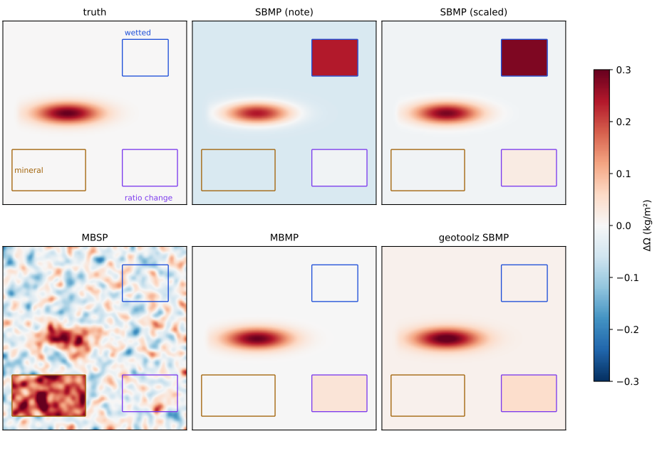
Figure 1:The truth and five retrievals on the same two-pass scene. Outlines: the stable mineral patch (brown), the wetted field (blue), the patch whose spectral ratio changed (purple).
Table 1:What each retrieval makes of the scene: the share of the plume’s mass it recovers, its offset over clean pixels, and each patch’s mean above the offset (kg/m²).
| Retrieval | Mass | Offset | Mineral | Wetted | Ratio change | Clean sd |
|---|---|---|---|---|---|---|
| SBMP, no scale factor (derivation 1) | 0.46 | −0.045 | 0.000 | 0.28 | 0.036 | 0.000 |
| SBMP, scene-wide | 0.86 | −0.011 | 0.000 | 0.29 | 0.035 | 0.000 |
| MBSP | 0.76 | −0.016 | 0.21 | 0.006 | 0.023 | 0.054 |
| MBMP, exact table, on background | 0.99 | −0.001 | 0.000 | 0.000 | 0.039 | 0.000 |
| MBMP, over every pixel (derivation 1) | 0.89 | −0.009 | 0.000 | 0.000 | 0.039 | 0.000 |
| MBMP, log ratio, linear in | 0.91 | −0.001 | 0.000 | 0.000 | 0.039 | 0.000 |
| MBMP, difference, linear in (derivation 1) | 0.88 | −0.001 | 0.000 | 0.000 | 0.039 | 0.000 |
| MBMP, difference, , (derivation 2) | 0.78 | −0.001 | 0.000 | 0.000 | 0.035 | 0.000 |
geotoolz plume.SBMP (with a reference), exact table | 1.16 | +0.013 | 0.000 | 0.000 | 0.040 | 0.000 |
We find the hierarchy the derivations describe (Figure 1, Table 1). SBMP, with or without a scale factor, reads the wetted field as 0.28 to 0.29 kg/m² of methane, which is nearly the plume’s peak. MBSP reads the stable mineral patch as 0.21 kg/m² and the 4 % ratio texture as 0.054 kg/m² of clutter. MBMP removes both, and the scene-wide brightening and the water-vapour change with them. What it keeps is the patch whose band ratio changed, where 3 % reads as 0.039 kg/m². The plume’s mass then depends on two choices which the derivations make differently. A scale factor fitted over every pixel takes in the plume, moves by 0.31 % and leaves a −0.009 kg/m² offset that costs 11 % of the mass. In addition, the slope that converts the signal to a column matters: the exact table recovers 99 %, a linear inversion 91 %, the difference 88 %, and with 78 %. geotoolz’s SBMP keeps the 1 % water-vapour change as a +0.013 kg/m² offset over the whole scene, which is 16 % extra mass on this plume (why).
Noise
TL;DR. Each ratio cancels a surface term and adds the noise of the bands it uses.
Problem. With independent noise of relative size in each band and pass, the log ratios add variances. SBMP uses two band-12 images, MBSP one image of each band and MBMP four images, and the two-band methods divide by the smaller . So, to first order, the standard deviations of the retrieved columns are
1 2 3# Shapes: obs, ref (2, 200, 200); ε = 0.01 per band and pass # sd(ΔΩ̂_noisy − ΔΩ̂_clean) off the plume (200, 200) → () # → SBMP 0.016, MBSP 0.018, MBMP 0.025 kg/m²; theory within 3 %
Retrieval noise for 1 % band noise on a stable surface, from a real run.
As (11) and (13) predict, MBMP pays for its robustness with 1.6 times SBMP’s noise. On a surface that is stable in time, SBMP with a scale factor is the more precise retrieval, and on a surface that is uniform in its band ratio, MBSP needs no reference pass. MBMP is the default because real surfaces are neither, and its noise falls with averaging whereas a surface artefact does not.
When MBMP is not the right choice
Derivation (1) lists three cases, and the run bears on each:
No good reference pass. MBMP and SBMP both need a plume-free date with the same surface. If the only reference is from another season, the local ratio changes grow, and MBSP (which needs no reference) may do better.
A strongly wavelength-dependent surface. Where varies widely across the scene, one fits it poorly. MBMP still cancels the stable part of (the mineral patch is 0.000 kg/m² above the offset), but the fitted is less well defined, and SBMP avoids the band ratio.
Water vapour that changes between passes. Band 12 has water-vapour lines. A scene-wide change is a scene-wide factor, which the per-pass absorbs. However, a change that varies across the scene (a front, terrain) is not absorbed, and it reads like a changed band ratio, where 1 % is 0.013 kg/m².
What each method cancels
Table 2 collects the run: what each method removes, what it leaves, and its noise.
Table 2:The family as a difference in differences, from the run.
| Method | Removes | Leaves | Noise (1 %) | Reference pass |
|---|---|---|---|---|
| SBMP | stable surface; scene-wide change (with ) | any local change in band 12 (wetted field: 0.29) | 0.016 | needed |
| MBSP | scene-wide change; the mean band ratio | the band ratio’s spatial texture (0.054) and stable patches (mineral: 0.21) | 0.018 | none |
| MBMP | stable surface, in both bands; scene-wide change; local changes that keep the band ratio | local changes of the band ratio (3 %: 0.039) | 0.025 | needed |
Where it lives in the stack
The package boundaries inventory lists the pieces: plumax’s radtran.nb_lut (build_nb_lut, lookup_nb, inject_plume) for the band tables, georeader’s read_srf for the real response functions (B11 from 1569 to 1658 nm and B12 from 2113 to 2286 nm at half maximum), and geotoolz’s plume.SBMP for the two-pass, two-band log signal. The scale factors, the background masks and the exact inversion exist nowhere in the stack, so we write them in the notebook.
Open questions
What should the operators be called? An
MBMPoperator in radtrax, withSBMPandMBSPbeside it, each with the scale factors and a background mask, would match the literature, and the currentSBMPcould become MBMP’sscale_factors=Falsemode.Where does the background mask come from? In the run, we use a first-pass detection grown by a Gaussian of 2 pixels. The alternatives are an iterated fit or the plume mask from geotoolz’s
PlumeMask, and the choice moves the offset.Should the band table include the background? plumax’s
nBomits it. Including it is one extra integral and changes band 12 by 1 % here, and more over a high background or long air-mass paths.
Upcoming work
Table 3 lists the follow-ups.
Table 3:Follow-ups from merging the two derivations.
| Follow-up | Where | Why |
|---|---|---|
Rename plume.SBMP (with a reference) to MBMP, and add per-pass scale factors | geotoolz now, radtrax after the move | it is an MBMP; without , a 0.013 kg/m² offset |
| Add SBMP and MBSP operators with scale factors fitted on a background mask | radtrax | the run: an all-pixel fit costs 11 % of the mass |
| Invert with the two-band table | radtrax, on plumax’s nb_lut | the run: 99 % of the mass against 91 % for the linear slope |
Build nB against the background column | plumax radtran.nb_lut | band model: 1.1 % on band 12 |
| Share the synthetic spectrum and band transmittance between radtrax · 1 and 2 | radtrax | both notebooks carry the same helpers |
References
The two derivations: “Deriving the MBMP method family from first principles” Johnson, 2026 and the step-by-step optical derivation Johnson, 2026.
The SBMP, MBSP and MBMP retrievals Varon et al., 2021; the IME and the fine-scale plume retrievals they feed Varon et al., 2018; a ground-truth calibration of Sentinel-2 retrievals Chen & others, 2022; transient emissions from geostationary observations Watine-Guiu et al., 2023.
geotoolz, georeader and plumax at the revisions in the header.
- Johnson, J. E. (2026). Deriving the MBMP Method Family from First Principles: from the radiative transfer equation to multi-band multi-pass methane retrieval. Unpublished design note.
- Johnson, J. E. (2026). An explicit optical derivation of the multi-band multi-pass (MBMP) method. Unpublished design note, generated with Gemini.
- Varon, D. J., Jervis, D., McKeever, J., Spence, I., Gains, D., & Jacob, D. J. (2021). High-frequency monitoring of anomalous methane point sources with multispectral Sentinel-2 satellite observations. Atmospheric Measurement Techniques, 14(4), 2771–2785. 10.5194/amt-14-2771-2021
- Varon, D. J., Jacob, D. J., McKeever, J., Jervis, D., Durak, B. O. A., Xia, Y., & Huang, Y. (2018). Quantifying methane point sources from fine-scale satellite observations of atmospheric methane plumes. Atmospheric Measurement Techniques, 11(10), 5673–5686. 10.5194/amt-11-5673-2018
- Chen, Y., & others. (2022). Detecting and quantifying methane emissions from oil and gas production: algorithm development with ground-truth calibration based on Sentinel-2 satellite imagery. Atmospheric Measurement Techniques, 15, 7155–7169.
- Watine-Guiu, M., Varon, D. J., & others. (2023). Geostationary satellite observations of extreme and transient methane emissions from oil and gas infrastructure. Proceedings of the National Academy of Sciences, 120(52).