The Beer–Lambert column retrieval
radtrax · 1 · From top-of-atmosphere reflectance to a methane column enhancement, term by term
Abstract
A methane plume over a bright surface removes a little bit of light in the short-wave infrared, and the single-layer Beer–Lambert model is how we turn that deficit into a column mass. In this page, we write the model out term by term, we say where each term comes from in a satellite product, and we follow the two ways one can estimate the plume-free baseline: a proxy band for multispectral sensors such as Sentinel-2, and a continuum fit for hyperspectral sensors such as EMIT. We then invert the model with a look-up table. The physics of the source note holds. However, five of its details do not: 1) Sentinel-2’s band 11 is not blind to methane, 2) the effective cross-section is only valid for weak absorption, 3) Sentinel-2 L1C has a radiometric offset, 4) Landsat L1 is not NetCDF or HDF5, and 5) the operational hyperspectral retrievals are matched filters, not continuum fits. On a synthetic Sentinel-2 scene, the note’s recipe recovers 80 % of the plume’s mass whereas the multi-band ratio with a look-up table recovers 96 %. radtrax (formerly rtmx) is the GeoModels package for radiative transfer in JAX, and it would own the band transmittance, the table and its inversion. A lot of this already exists in plumax (band-integrated radiative transfer, a HITRAN table pipeline, a matched filter), which the package boundaries page proposes to move.
About this page
| Status | Design. radtrax does not exist yet; this page fixes the physics its first module implements, and names what the stack and plumax already do |
| Reading time | about 25 minutes |
| Audience | anyone writing or reviewing a methane column retrieval, and anyone deciding what radtrax owns |
| Companions | radtrax · 2 (the multi-pass family and the MBSP estimator); radtrax · 3 (radtrax’s design); plumax · 1 (the emission rate from the column); the package boundaries page (where the code moves); Report 16 (one methane scene through geotoolz, with the matched filter and the IME); Report 9 (the use cases built on the same scene); Report 5 (pipelines under JAX, for a differentiable radtrax); Report 17 (the five-band sensor, a simpler Beer–Lambert model) |
| Code checked against | georeader-spaceml 2.4.1 (the Sentinel-2 L1C reader, its SRF table COPE-GSEG-EOPG-TN-15-0007 v4.0, the EMIT reader and the Gaussian SRF helper); geotoolz 0.10.2 at 088475e (plume, spectral, matched_filter); xrtoolz 0.0.5 at 308c7f2 (atm.gas.ch4). Read on 14 October 2026 |
| Running example | every number and figure is from one run of notebooks/geomodels/radtrax_01_column_retrieval.py, which builds the scenes from fixed seeds and asserts each number the page shows; code comments carry the status markers |
| Sources | the source note, “The Core Forward Model Equation” and its four companion sections Johnson, 2026; Varon et al. on Sentinel-2 Varon et al., 2021; Thompson et al. on the matched filter Thompson et al., 2015 |
The forward model
The reflectance a sensor measures in band at the pixel location is the surface reflectance times the transmittance of the two-way path through the atmosphere, averaged over the band’s spectral response on the spectral range :
Here is the methane cross-section per unit mass, is the background column and is the plume’s enhancement, and every symbol is a scalar (see Table 1). When every line is optically thin, the band average of the exponential is the exponential of the band-averaged cross-section, so (1) becomes the source note’s model:
where the band-averaged cross-section is
This means the plume’s optical depth is linear in the column:
(2) is the right picture for small plumes and the wrong one for strong lines. The running example measures how wrong it is in stage 2.
The variables
Table 1 gives each term of (1) with its shape, its units and the piece of the stack that supplies it. They are all scalars per band and per pixel, so none of them is bold; only the pixel location and the spectra of stage 5 are vectors.
Table 1:Every term of the model, where it comes from, and the stack piece that supplies it today.
| Symbol | Name | Role | Shape | Units | From | In the stack today |
|---|---|---|---|---|---|---|
| top-of-atmosphere reflectance | input | dimensionless | the L1 product | georeader’s Sentinel-2 L1C and EMIT readers | ||
| surface reflectance | nuisance | dimensionless | scene statistics, as part of the baseline | |||
| background transmittance (methane, water vapour, CO₂) | nuisance | dimensionless | scene statistics, or a radiative transfer model | |||
| two-way geometric air-mass factor | input | dimensionless | sun and view zenith angles in the metadata | georeader’s sza and vza grids (Sentinel-2) | ||
| spectral response of band | parameter | dimensionless | the agency’s SRF table | georeader’s read_srf (Sentinel-2) and srf (Gaussian) | ||
| , | mass absorption cross-section, and its band average | parameter | m²/kg | a line list, then the band’s response | georeader’s read_srf (Sentinel-2) and srf (Gaussian); plumax’s hapi_lut (HITRAN through HAPI) and radtran.srf | |
| background methane column | parameter | kg/m² | climatology or a model | xrtoolz’s dry_air_column and mixing_ratio_to_column | ||
| column mass enhancement | output | kg/m² | the inversion | geotoolz’s matched filter; xrtoolz’s column_mass_to_delta_vmr converts it |
On this page, is the methane column (as in the source note) and not a spatial domain, and is the surface reflectance and not an air density.
Where each term comes from
Each term has one source in a satellite product (Figure 1).
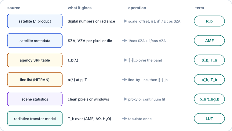
Figure 1:The sources of the model’s terms, from the notebook.
Reflectance. For Sentinel-2 L1C, the granule’s JPEG 2000 bands are top-of-atmosphere reflectance scaled to integers:
with a quantification value of 10,000 and, since processing baseline 04.00 (January 2022), an offset of −1,000. Hyperspectral L1 products are radiance instead, which we convert with the band’s solar irradiance and the Earth–Sun distance in astronomical units:
Air-mass factor. The geometric two-way path through a plane-parallel layer is
where and are the sun and view zenith angles.
Cross-section. A line list gives at the layer’s pressure and temperature. The band’s response function then averages it, (3), or, for the exact model, averages the transmittance, (1).
1 2 3 4 5 6 7 8 9 10 11# Shapes: S2 L1C tile (13, H, W); EMIT L1B (285, H, W); SRF table (877, 13) s2 = S2ImageL1C(safe_path) # today s2.quantification_value(), s2.radio_add_offsets() # 10000, {B12: -1000} today # R_b = (DN_b + offset_b) / Q R = s2.load() # reflectance today # AMF = 1/cos(SZA) + 1/cos(VZA), from the 5 km angle grids sza, vza = s2.sza, s2.vza["B12"] # GeoTensors today m = 1 / np.cos(np.radians(sza)) + 1 / np.cos(np.radians(vza)) # user # R_b = π L_b d² / (E_b cos(SZA)) emit = EMITImage(l1b_path); R_h = emit.load(as_reflectance=True) # today srf = read_srf("S2A") # B11, B12 at 1 nm, offline today
Reading the terms with the stack today.
The running example: one plume, two sensors
The scene is a 4 km × 4 km Sentinel-2 scene at 20 m, so 200 × 200 pixels. The surface has a smooth band 11 reflectance between 0.20 and 0.40 and two cover types, with band 12 at 0.84 and 0.80 of band 11 and a 1 % per-pixel scatter. A Gaussian plume, elongated and rotated by 30°, peaks at kg/m². The background is 1.9 ppm (a column of 0.0109 kg/m²), and the sun and view zenith angles are 35° and 5°, so (7) gives . Each band adds noise with a standard deviation of 0.0015 in reflectance. Stage 5 then adds an EMIT-like cube.
Stage 1 · The forward model (georeader → radtrax)
TL;DR. Build the exact model (1) with Sentinel-2’s own response functions.
1 2 3 4 5 6 7 8 9 10# Shapes: N_λ = 100,000 wavelengths (0.01 nm); H = W = 200 srf = read_srf("S2A") # (877, 13) at 1 nm today f11, f12 = np.interp(WL, srf.index, srf["B11"]), ... # (N_λ,) user # σ̄_b = ∫ f_b σ dλ / ∫ f_b dλ s11, s12 = band_mean(sigma, f11), band_mean(sigma, f12) # 0.04, 0.40 user # T_b(AMF, Ω) = ∫ f_b exp(−AMF σ Ω) dλ / ∫ f_b dλ T = radtrax.band_transmittance(sigma, f12) # (AMF, Ω) → T proposed (radtrax) # R_b = ρ_b T_b(AMF, Ω_bg + ΔΩ) + ε_b R12 = rho12 * T(m, OMEGA_BG + d_omega) + eps # (H, W) user # T₁₂(AMF, Ω_bg) = 0.990: the background takes 1 % of band 12
The forward model with Sentinel-2A’s band 11 and band 12, from a real run.
Sentinel-2A’s band 12 is above half its peak from 2113 to 2286 nm, and band 11 reaches 1668 nm. The background methane already removes 1 % of band 12’s light along this path.
Stage 2 · The effective cross-section against the exact band (radtrax)
TL;DR. Compare the linear optical depth (4) with the exact one, the curve of growth.
Problem. The plume’s exact band optical depth, above the background, is
where is the band transmittance of a column , and the linear model claims that . However, a line’s core saturates long before its wings do, so the band absorbs less than the linear model says.
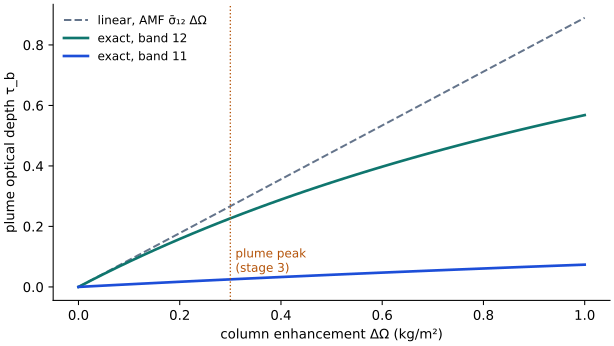
Figure 2:The curve of growth for band 12 and band 11, on the synthetic spectrum.
The exact optical depth (8) falls short of the linear one (Figure 2) by 3.8 % at 0.05 kg/m², by 15 % at the plume’s peak (0.3 kg/m², where band 12 dips by 20 % and not the 23 % the linear model gives), by 22 % at 0.5 and by 36 % at 1 kg/m². Band 11 absorbs about a tenth as much, which is simply the ratio we built this spectrum with.
Stage 3 · The multispectral proxy baseline (geotoolz, radtrax)
TL;DR. Estimate the plume-free band 12 from band 11 in two ways, invert linearly, and integrate the plume’s mass.
Problem. Under the plume, is unknown, but band 11 sees the same surface. There are two ways to use it. a) The source note fits on the pixels outside a suspected-plume mask and uses as the baseline, where are the intercept and the slope. b) The multi-band single-pass (MBSP) retrieval of Varon et al. Varon et al., 2021, whose estimator radtrax · 2 derives, fits through the origin over the whole scene with one ratio , and uses the fractional change
which, to first order, gives the column as
This keeps band 11’s own absorption. We score both by the plume’s mass above the median of a ring of clean pixels around it, as the integrated mass enhancement method does.
1 2 3 4 5 6 7 8 9 10# Shapes: H = W = 200; plume mask 3,777 pixels; true mass 108,979 kg # (a) R₁₂ ≈ θ₁ R₁₁ + θ₀ on clean pixels; τ = −ln(R₁₂ / (θ₁ R₁₁ + θ₀)) slope, intercept = np.polyfit(R11[~suspect], R12[~suspect], 1) # 0.816, 0.0016 user omega_a = -np.log(R12 / (slope * R11 + intercept)) / (m * s12) # B11 "blind" user # → 80 % of the mass # (b) R₁₁ ≈ c R₁₂ through the origin; ΔΩ = −ln(c R₁₂ / R₁₁) / (AMF (σ̄₁₂ − σ̄₁₁)) c = (R11 * R12).sum() / (R12 * R12).sum() # 1.220 user omega_b = -np.log(c * R12 / R11) / (m * (s12 - s11)) # user # → 89 % of the mass; noise off the plume 0.029 (a), 0.032 (b) kg/m² gz.plume.SBMP()(scene, reference_scene) # the multi-pass ratio today
Two proxy baselines on the Sentinel-2 scene, from a real run.
The note’s recipe loses a fifth of the plume, and there are two causes which add up. Band 11 absorbs under the plume, so the baseline is too low there by about of the signal (a tenth here), and saturation (stage 2) takes most of the rest. MBSP removes the first cause by subtracting , and it recovers 89 %. However, neither baseline can model the second surface cover. Its patches, where band 12 is 0.80 of band 11 rather than 0.84, come out as false enhancements of 0.04 kg/m² (Figure 3). So it is this surface term, not the sensor noise, that sets the noise floor.
Stage 4 · A look-up table of the band observable (radtrax)
TL;DR. Tabulate the MBSP observable exactly over the air-mass factor and the enhancement, and invert each pixel by interpolation.
Problem. We replace the first-order relation in (10) by the exact band observable
which we tabulate once, and then we solve for in each pixel.
1 2 3 4 5 6 7 8# Shapes: table (7, 81) over AMF ∈ [2, 3.5] and ΔΩ ∈ [0, 0.4] kg/m² # g(AMF, ΔΩ) from the exact band transmittances, both bands lut = radtrax.Table(observable="mbsp", sensor="S2A", m=np.linspace(2, 3.5, 7), omega=np.linspace(0, 0.4, 81)) proposed (radtrax) # ΔΩ = g⁻¹(−ln(c R₁₂ / R₁₁); AMF), odd-extended for negative noise omega_lut = lut.invert(-np.log(c * R12 / R11), m) # (H, W) proposed (radtrax) # → 96 % of the mass; RMSE over the plume 0.0175 kg/m² (linear: 0.0206)
Building and inverting the table, from a real run.
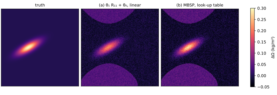
Figure 3:The truth, the source note’s recipe and MBSP with the table.
The table recovers 96 % of the mass. The remaining 4 % comes from the ring’s median, which the surface patches pull below zero. Because of (11) is increasing in at every in the table, the inversion is a one-dimensional interpolation. The note’s table has water vapour as a second index. That matters where water and methane lines overlap in band 12, but this synthetic spectrum has no water, so it does not test it.
Stage 5 · Hyperspectral: a continuum against a matched filter (georeader, geotoolz)
TL;DR. On an EMIT-like cube, fit the note’s quadratic continuum and compare it with geotoolz’s matched filter, over a surface with a carbonate absorption.
Problem. The cube is 120 × 120 pixels with bands from 2000 to 2500 nm, 7.4 nm apart with an 8.5 nm full width at half maximum. The surfaces follow a quadratic in wavelength, and 15 % of the pixels carry calcite’s absorption near 2340 nm, which is inside the methane band. The plume peaks at 0.15 kg/m². Again we compare two approaches. a) The note’s continuum is a quadratic per pixel through the windows from 2120 to 2150 nm and from 2430 to 2470 nm, followed by a least-squares column over the 27 bands from 2200 to 2400 nm. b) The matched filter Thompson et al., 2015 estimates the enhancement at pixel from its spectrum as
where and are the background mean and covariance of the spectra, and is the linearised target (the Jacobian of (2) with respect to at , with the band-averaged cross-sections of all the bands). The estimate is a scalar per pixel.
1 2 3 4 5 6 7 8 9 10 11 12# Shapes: cube (N_Sy, H, W) = (68, 120, 120); 9 window bands, 27 fit bands srf_h = reflectance.srf(centres, fwhm, WLH) # (N_λ, N_Sy) Gaussian today # (a) R / (θ₂ λ² + θ₁ λ + θ₀) fitted on the windows; ΔΩ by least squares omega_cont = continuum_column(cube, windows, fit) # (H, W) user # (b) ΔΩ̂ = J_hᵀ Σ_y⁻¹ (y − μ_y) / (J_hᵀ Σ_y⁻¹ J_h), J_h = −AMF μ_y ⊙ σ̄ mf = gz.matched_filter.MatchedFilter(target=j_h, fit_on_call=True, axis=0) # today omega_mf = mf(cube) # background includes the plume today masked = cube.copy(); masked[:, suspect] = np.nan # NaN: left out of the fit mf_bg = gz.matched_filter.MatchedFilter(target=j_h, axis=0).fit(masked) # today omega_mf_bg = mf_bg.transform(cube) # today # mass: continuum 95 %, matched filter 72 % (plume in Σ_y), 91 % (masked) # over carbonate: continuum +0.0069, matched filter +0.0002 kg/m²
The continuum fit and geotoolz’s matched filter on the cube, from a real run.
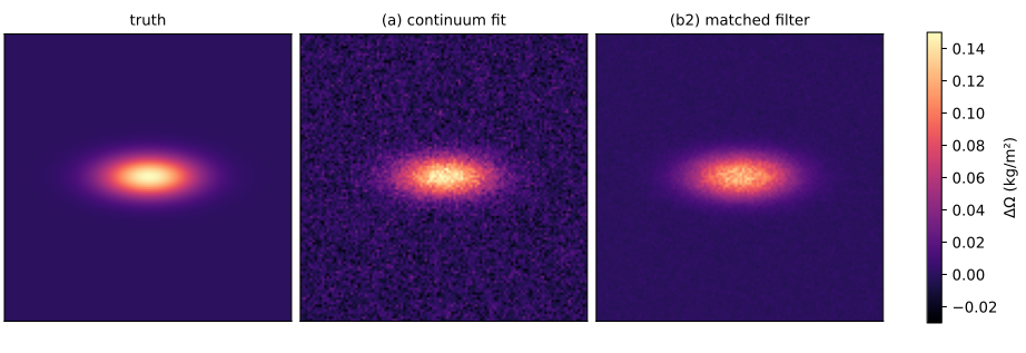
Figure 4:The truth, the note’s continuum fit and the matched filter with the plume left out of its background.
The continuum fit recovers 95 % of the mass, but it reads carbonate as methane (Figure 4): the pixels with calcite come out 0.0069 kg/m² high, against 0.0029 kg/m² low over the rest, and its noise off the plume is 0.0095 kg/m². The matched filter (12) learns the carbonate from the scene covariance and leaves no bias there (0.0002 kg/m²), with a noise of 0.0016 kg/m². Its one trap is the plume itself. With the plume inside the background statistics, the filter only recovers 72 % of the mass, whereas with the suspected plume masked out of the fit it recovers 91 %. The rest is saturation, as in stage 2, because the target is linearised. At the peak, 0.15 kg/m² mixed over a 500 m layer is a 442 ppm enhancement (xrtoolz’s column_mass_to_delta_vmr).
What radtrax would own
Where each piece lives today is in the package boundaries inventory, and Table 2 keeps what radtrax would hold.
Table 2:Each step of the retrieval and what radtrax would hold.
| Step | radtrax (proposed) |
|---|---|
| read reflectance, offsets, angles | stays in georeader |
| response functions | one band-integration operator, reading georeader’s tables through [geo] |
| cross-sections from a line list | moved from plumax hapi_lut |
| band transmittance | moved from plumax radtran.forward, with the background column of (1) |
| baselines | SBMP moved from geotoolz, and the single-pass MBSP observable (9) |
| table and inversion | Table over , monotone inversion, in place of plumax’s radtran.nb_lut |
| matched filter | one core, merged from the three |
| variational retrieval | moved from plumax assimilation, or split with vardax (open) |
| units, mass and rate | stay in xrtoolz; the plume operators go to plumax |
Written in JAX, the band transmittance is differentiable, so the table becomes optional. A Gauss–Newton step on (1) inverts each pixel directly, as the Laplace step of Report 17 does on the five-band sensor, and one can train a learned retrieval through it (Report 5).
Open questions
Are the note’s continuum windows clean? The windows from 2120 to 2150 nm and from 2430 to 2470 nm need checking against HITRAN’s methane and water lines at EMIT’s resolution, and the long-wave window sits at the edge of methane’s 2.3 μm band.
Which band 11 to band 12 ratio does Sentinel-2 really have? The bias of stage 3 scales with . The tenth we use here is a choice, and the real ratio follows from HITRAN and the two response functions.
A table or a solver? A table is fast and auditable, whereas a differentiable forward model is exact at every pixel and composes with learning. radtrax could ship both, with the table built from the forward model.
Which atmosphere? The single layer with a geometric air-mass factor ignores scattering and the vertical profile. When does a layered model pay for itself on Sentinel-2’s bands?
Upcoming work
Table 3:Follow-ups from checking the source note.
| Follow-up | Where | Why |
|---|---|---|
| Rerun the example on HITRAN lines | this page’s notebook, with a cached line list | the spectrum here is synthetic |
| Add the single-pass MBSP observable | radtrax (or geotoolz plume until radtrax exists) | stage 3: the stack has no single-pass proxy |
| Ship a Landsat L1 reader path with the MTL scaling and angle bands | georeader | the note’s Landsat route does not exist in the stack |
References
The source note on the forward model, provenance, proxies and look-up table Johnson, 2026.
Varon et al. on Sentinel-2 methane retrievals Varon et al., 2021, and on the integrated mass enhancement Varon et al., 2018.
Thompson et al. on the matched filter for imaging spectroscopy Thompson et al., 2015.
georeader-spaceml, geotoolz and xrtoolz at the revisions in the header.
- Johnson, J. E. (2026). The Core Forward Model Equation: a Beer–Lambert methane retrieval, its inputs, proxies and look-up table. Unpublished design note.
- Varon, D. J., Jervis, D., McKeever, J., Spence, I., Gains, D., & Jacob, D. J. (2021). High-frequency monitoring of anomalous methane point sources with multispectral Sentinel-2 satellite observations. Atmospheric Measurement Techniques, 14(4), 2771–2785. 10.5194/amt-14-2771-2021
- Thompson, D. R., Leifer, I., Bovensmann, H., Eastwood, M., Fladeland, M., Frankenberg, C., Gerilowski, K., Green, R. O., Kratwurst, S., Krings, T., Luna, B., & Thorpe, A. K. (2015). Real-time remote detection and measurement for airborne imaging spectroscopy: a case study with methane. Atmospheric Measurement Techniques, 8(10), 4383–4397. 10.5194/amt-8-4383-2015
- Varon, D. J., Jacob, D. J., McKeever, J., Jervis, D., Durak, B. O. A., Xia, Y., & Huang, Y. (2018). Quantifying methane point sources from fine-scale satellite observations of atmospheric methane plumes. Atmospheric Measurement Techniques, 11(10), 5673–5686. 10.5194/amt-11-5673-2018