The state catalog
Report 13 · Indexing model states, reassessed against geocatalog, xrtoolz and pipekit-cycle
Abstract
A model state is a field which a model produced: an analysis, a forecast step, or one ensemble member of a reanalysis. Unlike an observation, it has two times (when the run started and when the state is valid), a member index, a producer and a parent state. The scoping report proposed statecatalog, a new sister package with its own slice, backends and queries for these states. However, when we read the pinned code, we find that most of that package already exists in pieces: geocatalog rows can carry the extra columns and filter on them, xrtoolz scores forecasts by lead time and by ensemble, and pipekit-cycle keeps the trajectory in memory. What is missing is narrower, namely typed state columns, loading that keeps runs apart, a handful of queries, forecast alignment and an ensemble history, plus area weighting when producers run on different grids (as in a CMIP ensemble). This report recommends building those pieces where their concepts already live, and not building statecatalog.
About this report
| Status | Redesign of a scoping proposal (“committed”: a sister package statecatalog). The user asked for it to be reassessed against the geotoolz and xrtoolz stacks; the recommendation below replaces the package |
| Reading time | about 30 minutes |
| Audience | anyone who stores, queries or scores forecasts, analyses or reanalyses with the stack |
| Companions | Report 6 (geocatalog); Report 3 (xrtoolz and the sister libraries); Report 9 (use cases); Report 10 (pipekit-cycle); Report 16 (the stack rules) |
| Code checked against | the revisions pinned in references/: pipekit and its sister packages at 0.0.2 (ef3c17f); geotoolz 0.10.2 with geocatalog 0.5.1 (088475e); xrtoolz 0.0.5 with xrreader 0.0.4 (308c7f2); pandas 3.0.6, as in pixi.lock. Read on 13 October 2026 |
| Running example | every output in the code blocks is from real runs over two synthetic archives: an 11-file regional forecast archive (stages 1 to 5) and a 6-file, three-model archive on three grids (stage 6); both are described in Section ??, and notebooks/reports/report13_state_catalog.py regenerates them from fixed seeds and asserts every number shown |
Summary
Decision. Model states are indexed by geocatalog, through a new geocatalog.states namespace over the existing backends, and they are scored by xrtoolz’s existing forecast metrics. There is no statecatalog package, no StateSlice and no second GeoParquet format, and we update the overview to match in the same change. No library starts importing another: pipekit-cycle, geocatalog and xrtoolz stay independent, and scripts join them.
A. State columns in geocatalog. Today a forecast’s run time and member can live in extra columns, but nothing names, types or fills them. So we reserve five columns in schema v1 and add a builder that reads them from CF or cfgrib metadata.
B. Run-aware loading and typed queries.
load_xarrayconcatenates on time and drops duplicates, so overlapping runs lose steps silently. We addload_states, which stacks files into an (init time, member, lead time) cube (or into anxr.DataTreewith one leaf per producer when producers use different grids), and typed query functions which replace hand-writtenwherestrings.C. Forecast alignment in xrtoolz.
SkillByLeadTimeandCRPSscore a forecast cube today. However, the caller builds the verifying reference by hand, and pixel metrics cannot reduce over a dimension which the reference lacks. So we addalign_reference, broadcast the reference in the pixel metrics, and letgeo.Reduceweight by cell area, so that multi-model area means need no user code.D. Ensemble histories in pipekit-cycle.
CycleandDACyclekeep their trajectory inhistory, whereasEnsembleCycleandEnsembleDACyclekeep nothing. We addsave_historyto both, and writing files stays in scripts, as AGENTS.md requires.
End state. A script runs a cycle and writes one file per run and member. geocatalog indexes the files with typed state columns and loads them back as a cube without mixing runs, and xrtoolz aligns the cube with its analyses and scores it by lead time. Runs from several models on several grids load as a tree, they are summarised on their own grids, and they are only regridded conservatively for the comparison. pipekit-experiment’s Run.pipeline_hash names the producer. Every one of the scoping report’s queries is either a function in geocatalog.states or an existing call.
The problem, as the scoping report put it
An observation has one time. A model state has several, and the scoping report named them well. Let be the run time (the initialisation time of a forecast) and the valid time (the time the state describes), where both are time stamps on the time axis , and let
be the lead time ((1)), a scalar . An analysis is the state which a data-assimilation step produces at its own valid time, so . A forecast run started at produces states at for a model step . An ensemble repeats each run times, with members indexed . In addition, each state has a producer (the hash of the model and configuration that made it) and its parents (the states it was computed from). A forecast has one parent, the state its run started from, whereas an ensemble-Kalman analysis has the whole forecast ensemble as its parents, because its gain is estimated from all members at once. Table 1 lists each field with its CF name and where it lives today.
Table 1:The fields of a model state, their CF names and where each one lives today.
| Field | Symbol | CF / cfgrib name | CMIP6 attribute | Today |
|---|---|---|---|---|
| Valid time | time, valid_time | time | geocatalog’s row interval (start_time, end_time) | |
| Run time | forecast_reference_time / cfgrib time | an extra column, if the user adds it | ||
| Lead time | forecast_period / cfgrib step | derived; xrtoolz’s lead_dim="lead_time" | ||
| Member | realization / cfgrib number | member_id, a variant label such as r1i1p1f1 | an extra column; xrtoolz’s ensemble_dim="member" | |
| Producer | source_id | Run.pipeline_hash in pipekit-experiment; an extra column in the catalog | ||
| Parents | , a set | nowhere |
The questions which the scoping report wanted answered are the right ones: 1) which states are valid at a time, 2) what the latest analysis before a time is, 3) which states one run produced, 4) which members share a run, 5) what a state descends from, and 6) which observations an analysis assimilated. The rest of this page answers each one with the code that exists, and we add what is missing.
Ownership rules
States are produced by pipekit-cycle, indexed by geocatalog and scored by xrtoolz, and only scripts join the three (Figure 1).
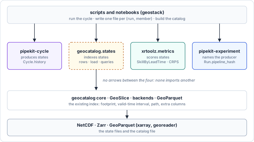
Figure 1:Ownership of model states. The dashed box is the only new namespace; the other three already ship.
geocatalog owns the index of states (geocatalog.states), which means the reserved columns, the state builder, run-aware loading and the state queries. It never imports pipekit or xrtoolz.
The other three follow the stack rules: pipekit-cycle produces states in memory and writes no files, xrtoolz verifies them, and pipekit-experiment names the producer (Run.pipeline_hash). None of them imports another, and scripts own every side effect.
The running example: a regional methane forecast archive
The archive. A regional methane system covers a 4 × 4 grid over the Permian Basin (31° to 34° N, 104° to 101° W), which is the state grid with cells indexed by . Each day, it runs one data-assimilation step which writes an analysis of the column-methane anomaly field in ppb, at location and time , and we write for the analysis at valid time in grid cell . From each of the first three analyses, it launches a two-member ensemble forecast with leads of 0, 1 and 2 days. So the archive holds 5 analysis files and forecast files (one per run and member, with the number of runs), and each of them is NetCDF with a time axis of valid times. Each file’s attributes record its kind, run time, member, producer hash and parent file.
The data. The truth is a random walk in time, and the analyses add noise with a standard deviation of 0.05 ppb, whereas the forecast error grows with lead as (with in days and in ppb). The data are synthetic, so we can check the scores in stage 4 against their expected values.
The notebook notebooks/reports/report13_state_catalog.py builds the archive from a fixed seed in a temporary directory, runs every stage, and asserts each number on this page, and it runs with geocatalog 0.5.1 and xrtoolz 0.0.5 from references/. Stage 6 widens the example from one regional system to a multi-model comparison, with its own six-file archive in the same notebook. The blocks below are excerpts with their real outputs, and names such as cat, t3 and five_days are defined in the notebook. Lines marked user (markers) are glue which the workstreams remove.
Stage 1 · Index the archive (scripts → geocatalog)
TL;DR. Index the eleven files so that later questions never open a file.
Problem. Each file has a footprint, a valid-time interval and a path, which geocatalog’s xarray kind already records. However, a state index also needs the run time , the member , the producer and the set of parents on every row.
1 2 3 4 5 6 7 8 9 10 11 12 13 14# Shapes: N_run = 3 runs, N_e = 2 members, N_lead = 3 leads, H = W = 4 cells; 11 files from geocatalog.build import build_xarray_catalog from geocatalog.storage import from_geoparquet, to_geoparquet # one row per file: footprint, [v_min, v_max], path cat = build_xarray_catalog(paths, crs="EPSG:4326") # 11 files → 11 rows today # r(f), e(f), h(f), P(f): read from the file attributes attrs = [xr.open_dataset(p).attrs for p in cat.gdf.filepath] # user cat.gdf["run_time"] = pd.to_datetime([a["run_time"] for a in attrs]) # user cat.gdf["member"] = [int(a["member"]) for a in attrs] # user cat.gdf["producer"] = [a["producer"] for a in attrs] # user cat.gdf["parent_uri"] = [a["parent_uri"] for a in attrs] # user to_geoparquet(cat, "states.parquet") # extras kept today cat = from_geoparquet("states.parquet") # run_time datetime64 today
Index the archive with today’s xarray builder, then copy the state fields into extra columns.
The extra columns survive the GeoParquet round trip with their types (run_time as datetime64[us], member as int64), because geocatalog keeps every non-reserved column in CatalogRow.extras. What does not exist is a builder that fills them. The xarray builder reads neither forecast_reference_time nor realization, and a file without a time coordinate gets the placeholder interval 1900 to 2100 with n_timesteps=0. Workstream A adds the builder and reserves the names.
Stage 2 · Ask the scoping report’s questions (geocatalog)
TL;DR. Find one run’s forecasts, the latest analysis before a time, and the members of a run, using only the index.
Problem. With the set of rows, the three questions are the filters (2), (3) and (4):
where is a run time, is a member and is the query time, so the first filter returns a set of rows, the second one row and the third a set of members.
1 2 3 4 5 6 7 8 9 10 11 12 13 14 15# chain(r₀ = 01-02, e₀ = 0) cat.where("kind == 'forecast' and member == 0 and run_time == '2026-01-02'") # → 0 rows: a string equality on a datetime column matches nothing today cat.where("kind == 'forecast' and member == 0" " and run_time >= '2026-01-02' and run_time < '2026-01-03'") # → ['fc_20260102_m0.nc'] today # latest(01-03 06Z): end times live in the IntervalIndex after a round trip ana = cat.where("kind == 'analysis'").gdf # today ana = ana[ana.index.right <= pd.Timestamp("2026-01-03 06:00")] # user ana.iloc[ana.index.right.argmax()].filepath # → 'ana_20260103.nc' user # members(r₀ = 01-01) cat.where("kind == 'forecast' and run_time < '2026-01-02'").gdf.member # → [0, 1] today
The three questions as where strings over the extra columns, with their outputs.
Every answer is right, but each one is a string which the user must get exactly right. The first query shows why that matters: on pandas 3.0.6 (the version in pixi.lock), DataFrame.query("t == '2026-01-02'") on a datetime column returns no rows, whereas df[df.t == "2026-01-02"] returns one, and nothing warns about the miss. Typed functions which take a pd.Timestamp (workstream B2) remove the trap.
Stage 3 · Load a forecast cube (geocatalog → xarray)
TL;DR. Load the six forecast files as one array indexed by run, member and lead.
Problem. The cube which xrtoolz expects is (5),
whose entry is member of run at lead in cell , with leads and the cells laid out on the grid. The valid time is a two-dimensional coordinate. Three runs overlap in valid time, since all three are valid on 3 January, at leads 2, 1 and 0.
1 2 3 4 5 6 7 8 9 10 11 12 13 14 15 16 17 18 19 20 21# Shapes: N_run = 3, N_e = 2, N_lead = 3, H = W = 4 from geocatalog import GeoSlice from geocatalog.load import load_xarray rows = cat.where("kind == 'forecast'").gdf # 6 rows today jan3 = GeoSlice(bounds=(-104.5, 30.5, -100.5, 34.5), interval=pd.Interval(t3, t3, closed="both"), resolution=(1.0, 1.0), crs="EPSG:4326") # today m0 = cat.where("kind == 'forecast' and member == 0").query(jan3) # 3 rows today load_xarray(m0, jan3).sizes["time"] # → 1: two runs dropped today # x⁽ᵉ⁾_n(r, τ): one file per (r, e), relabelled from v to τ = v − r pieces = [] for (r, m), row in rows.set_index(["run_time", "member"]).iterrows(): # user ds = xr.open_dataset(row.filepath).load() # user ds = (ds.assign_coords(lead_time=("time", ds.time.values - r)) # user .swap_dims(time="lead_time").drop_vars("time")) # user pieces.append(ds.expand_dims(init_time=[r], member=[m])) # user fc = xr.combine_by_coords(pieces, combine_attrs="drop") # user fc = fc.assign_coords(valid_time=fc.init_time + fc.lead_time) # user # → sizes {'init_time': 3, 'member': 2, 'lead_time': 3, 'lat': 4, 'lon': 4}
Today’s loader keeps one run per valid time; the cube has to be stacked by hand.
load_xarray is right for observations, where two files covering the same time are duplicates. However, for forecasts the same valid time from two runs is two different states, and drop_duplicates on time keeps one of them without a warning. The eight user lines are the cube builder which workstream B1 puts in load_states.
Stage 4 · Score the forecasts by lead time (xrtoolz)
TL;DR. Compare each forecast with the analysis valid at the same time, and report the error at each lead.
Problem. The verifying reference for run at lead is the analysis at its valid time, , which we stack into . With the ensemble mean over members and the number of scored values per lead, the two scores are (6) and (7),
with the CRPS of an ensemble as in the overview ((15)), so both scores are scalars in ppb at each lead. For this archive, the expected ensemble-mean RMSE is , which is 0.087, 0.427 and 0.779 ppb at leads 0, 1 and 2 days.
1 2 3 4 5 6 7 8 9 10 11 12 13 14 15 16 17 18# Shapes: X (N_run, N_e, N_lead, H, W); Y (N_run, N_lead, H, W) from xrtoolz.metrics import CRPS, RMSE, SkillByLeadTime an = load_xarray(cat.where("kind == 'analysis'"), five_days) # (T = 5, H, W) today # y_n(r, τ) = a_n(r + τ) ref = an.sel(time=fc.valid_time).drop_vars("time") # → (N_run, N_lead, H, W) user dims = ("init_time", "lat", "lon") # RMSE(τ) of the ensemble mean SkillByLeadTime(RMSE("xch4", dims=dims))(fc.mean("member"), ref) # → (N_lead,) today # → [0.076, 0.467, 0.746] # CRPS(τ) over members SkillByLeadTime(CRPS("xch4", ensemble_dim="member", dims=dims))(fc, ref) # today # → [0.048, 0.356, 0.605] # per-member RMSE: reduce over the member dimension too SkillByLeadTime(RMSE("xch4", dims=("member", *dims)))(fc, ref) # today # → ValueError: tuple.index(x): x not in tuple SkillByLeadTime(RMSE("xch4", dims=("member", *dims)))(*xr.broadcast(fc, ref)) # → [0.109, 0.617, 1.132] user
Align the analyses with the cube, then score by lead with today’s xrtoolz metrics.
The measured RMSE (0.076, 0.467 and 0.746) sits within sampling error of the expected values, with cells per lead. The per-member RMSE matches its expected , which is 0.112, 0.602 and 1.101. So the scoring is shipped, and what is missing is the alignment line (workstream C1) and the broadcast which lets pixel metrics reduce over a dimension that only the forecast has (C2).
Stage 5 · Trace lineage and the assimilation window (geocatalog)
TL;DR. Follow a state back through the runs it came from, and find the observations an analysis used.
Problem. With the set of parents of the state in row , the lineage of is every state we reach by following parents (, , , and so on) until no state has parents left. This is a directed acyclic graph, which is a chain when every state has one parent. This archive is the simple case, where each analysis lists one parent (the member-0 forecast). An ensemble-Kalman analysis would list every forecast member, because its gain is computed from all of them. For an analysis at time with an assimilation window of width , the observations used are the rows of an observation catalog whose valid time falls in .
1 2 3 4 5 6 7 8 9 10 11 12 13# f, P(f), P(P(f)), … until P = ∅; one parent per state in this archive by_uri = cat.gdf.set_index("filepath") # user uri, chain = "ana_20260104.nc", [] # user while uri: # user chain.append(uri) # user uri = by_uri.loc[uri, "parent_uri"] # user # → ana_20260104 ← fc_20260103_m0 ← ana_20260103 ← fc_20260102_m0 # ← ana_20260102 ← fc_20260101_m0 ← ana_20260101 # obs with v ∈ [t − w/2, t + w/2] # arguments sketched window = GeoSlice(bounds=aoi, interval=pd.Interval(t - w / 2, t + w / 2, closed="both"), resolution=res, crs="EPSG:4326") # today obs_used = obs_cat.query(window) # (M rows) today
Lineage is a walk over the parent column; the assimilation window is an ordinary query on the observation catalog.
The lineage walk is five lines of user code when each state has one parent, and a graph search when states have several. The scoping report’s assimilation_window needs no new code, since it is GeoCatalog.query with the window as the interval, or matchup with WithinWindow(start, end) when many analyses are matched at once. Workstream B2 adds lineage, and the window stays an existing call.
Stage 6 · Many producers on many grids: a CMIP-style comparison (geocatalog → xrtoolz)
TL;DR. Compare models that run on different grids, either by computing each model’s statistics on its own grid or by regridding all of them to one grid first, and see when the two give different answers.
Problem. A multi-model ensemble such as CMIP6 Eyring et al., 2016 holds runs from many models , with models. In CMIP6 terms, the model is the source_id, a run is a member_id (a variant label such as r1i1p1f1), and each model writes on its own grid (grid_label). Model has members and a grid of cells , where cell is the region with area , and its field is at day . The archive here is synthetic: model A on a 1° grid with 3 members, B on 2.5° with 1, and C on 2° with 2, 90 days each, with independent cell-scale weather of standard deviation 2 K on a zonal climatology. The six files are indexed like stage 1, with producer and member columns.
The area mean of a field on a grid with cells is the scalar , with the value in cell . A conservative regrid onto a common grid with cells and areas weights each source cell by its overlap , so that the area mean survives whenever the common grid covers the source grid:
A statistic over time and members, applied cell by cell, either commutes with or it does not. The time mean is linear, so . However, the 99th percentile (the sample quantile of each cell’s values) is not, because averaging cells before taking the percentile removes the cell-scale extremes that the percentile measures. That gives the three pipelines (10), (11) and (12):
where (3) equals (1) by (9), and (2) only equals (1) when is linear. Pipeline (3) is the usual way to draw a multi-model map, since each statistic is computed where the model resolved it and only the result is regridded. Combining the models needs one more choice, which is either one vote per model, , or one vote per member, , where both are scalars in K.
1 2 3 4 5 6 7 8 9 10 11 12 13 14 15 16 17 18 19 20 21 22 23 24 25 26 27 28 29# Shapes: N_K = 3 models; model k: (N_k, T = 90, H_k, W_k), H_k × W_k its own grid from xrtoolz.interpolate import RegridConservative # one leaf per producer, members stacked inside it; the grids differ leaves = {} for k, rows in cat.gdf.groupby("producer"): # user runs = [xr.open_dataset(p).load() for p in rows.filepath] # user leaves[f"/{k}"] = xr.concat(runs, dim="member") # user tree = xr.DataTree.from_dict(leaves) # today # → A (3, 90, 180, 360) · B (1, 90, 72, 144) · C (2, 90, 90, 180) # 𝓡: conservative regrid of every leaf onto the coarsest grid (2.5°) regrid = RegridConservative(grid_25, mode="mean", normalize="destarea") # today common = regrid(tree) # every leaf → (N_k, 90, 72, 144) today # ⟨x⟩ = Σₙ |cₙ| xₙ / Σₙ |cₙ|, with |cₙ| ∝ sin φₙ₊ − sin φₙ₋ def area_mean(y): ... # user # S = time mean (linear): (1) and (2) agree # → native A 277.9999 · B 279.4971 · C 277.2991 K # → regridded A 277.9999 · B 279.4971 · C 277.2991 K (max difference 1.2e-11) # S = F̂⁻¹(0.99) − time mean (nonlinear), per cell, then ⟨·⟩ # → (1) native A 4.289 · B 4.279 · C 4.288 K # → (2) regrid first A 1.544 · B 4.279 · C 2.564 K # → (3) hybrid A 4.289 · B 4.279 · C 4.288 K (equals (1) to 1.2e-11) # one vote per model vs one vote per member, S = time mean # → 278.2654 K vs 278.0159 K
Three models on three grids, loaded as a DataTree and compared three ways, from a real run.
The tree, the regrid and the map over models all ship today: xrcore’s Operator maps any xrtoolz operator over the leaves of an xr.DataTree, and RegridConservative keeps area means to 1.2e-11 K across a 1° to 2.5° and a non-nested 2° to 2.5° regrid. The numbers show why the order of operations matters. Regridding first leaves the time mean untouched, but it removes 64 % of model A’s warm extremes and 40 % of model C’s, so the fine models look less extreme than the coarse one only because they were averaged. Model B is unchanged because it is already on the common grid. Two things are user code: 1) grouping the catalog into leaves, which workstream B1 adds as load_states(..., group_by="producer"), and 2) the area mean, which geo.Reduce cannot weight (workstream C3). The vote is a choice which the script must state, and here it moves the ensemble mean by 0.25 K.
Comparing each model with observations runs the other way, where the observations are regridded onto each model’s native grid so that the statistic is computed where the model resolved it. RegridConservative and RegridLike take their target grid when they are built, so today that is one operator per leaf, built in a loop (regrid_conservative(obs, leaf) inside xr.map_over_datasets does the same). This is also the step where a pipekit Graph earns its place, since two inputs (the model leaf and the observations) feed one bias operator.
The scoping report’s names, checked
Table 2 checks every stack name the scoping report’s examples use.
Table 2:Every stack name the scoping report’s examples use, at the pinned revisions.
| Name in the report | At the pinned revisions |
|---|---|
statecatalog, StateSlice, StateRow, StateCatalog | not built; named only in pipekit-train’s design docs (architecture.md, api/datasets.md) |
InMemoryStateCatalog, DuckDBStateCatalog | not built; geocatalog’s InMemoryGeoCatalog and DuckDBGeoCatalog hold extra columns and filter them with where and sql |
CycleStateWriter, CycleStateReader | not built; see Section ?? |
pk.config_hash(op) | does not exist; pipekit_ops.hashing.sha256_hex(stable_json(op.get_config())) computes it, and Report 9 proposes pipeline_hash(op) (proposal B) |
georeader.read_from_url | does not exist; states are xarray files, read with xr.open_dataset or geocatalog’s load_xarray |
pc.Sequential | does not exist. pipekit_ops.Sequential threads a carry state when it holds stateful steps, but it is not a StatefulOperator, so Cycle(step_op=pk.Sequential([...])) raises TypeError: step_op must be a StatefulOperator or a ForwardModel even then (Report 10) |
pc.EnsembleCycle(step_op, n_steps, n_members) | exists, with that signature |
pt.SimulationDataset | exists, but simulates on the fly from a forward model and a prior; it reads no stored states |
Current-state audit
We checked eleven pieces of the proposed package: seven are healthy as they ship, three are split between a library that has them and a gap, and one is missing (Table 3), and Figure 2 counts the page’s calls by marker. The audit read the revisions pinned in references/ on 13 October 2026.
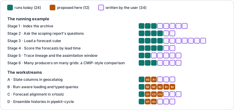
Figure 2:What this page’s sketches call: of 70 stack calls, 24 run today, 12 are proposed by this report’s workstreams and 34 are code the reader writes (how to read it).
Table 3:What each piece of the proposed statecatalog maps to today.
| Symbols | Defined in | Used by | Verdict |
|---|---|---|---|
bounds, CRS, valid-time interval; query, GeoSlice | geocatalog (InMemoryGeoCatalog.query, DuckDBGeoCatalog.query) | every catalog workflow | Healthy. Answers “valid at ” at file granularity |
extra columns; CatalogRow.extras; where, sql | geocatalog._src.base, backends.memory, backends.duckdb_backend | STAC extra_properties, user filters | Healthy. Holds , , , , but untyped and unnamed |
xarray builder; build_xarray_catalog(time_var=...) | geocatalog._src.formats.xarray_backend | xarray-kind catalogs | Split ownership. One row per file; reads no forecast metadata |
loader; load_xarray | same module | xarray-kind catalogs | Split ownership. Right for observations; for forecasts, drops overlapping runs (Section ??) |
schema versioning; SCHEMA_VERSION_CURRENT = 0, parquet._MIGRATIONS | geocatalog._src._schema, storage.parquet | GeoParquet round trip | Healthy. No migration registered yet; a reserved column is the first |
temporal matching; NearestInTime, WithinWindow, Synchronous, matchup | geocatalog._src.matchup | matchup tables | Healthy. Covers the assimilation window, on row midpoints |
lead-time skill; SkillByLeadTime, skill_by_lead_time | xrtoolz.metrics._src.forecast | viz.validation.LeadTimeSkillPanel, FacetPanel | Healthy. Needs a reference aligned on lead_dim, or none on it |
ensemble scores; CRPS, SpreadSkillRatio, RankHistogram, EnsembleCoverage | xrtoolz.metrics (ensemble_dim="member") | Healthy. Pixel metrics such as RMSE cannot reduce over member when the reference lacks it | |
trajectories; Cycle.history, DACycle.history | pipekit_cycle.cycle, pipekit_cycle.da | Split ownership. In memory; EnsembleCycle, EnsembleDACycle, SmootherCycle and WindowedCycle keep none | |
producer identity; Run.pipeline_hash, ModelRegistry.store, sha256_hex | pipekit_experiment.run, .registry; pipekit_ops.hashing | TrainingArtifact, InferenceArtifact | Healthy. The hash a row’s producer column records |
| lineage, forecast chains, typed state queries | Missing. Nothing anywhere |
Smaller findings:
A plain
Cycledoes not advance time._ForwardModelAdapterpasses the carry state through unchanged, soDAState.tstays 0.0, and only the DA cycles call_advance_da_state. So a history entry’s valid time must be computed from its index, where entry with a stride of steps is valid at (checked: a 4-stepCyclewith stride 2 keeps the states after steps 1 and 3).EnsembleCyclethreads one carry state through all members. Its loop callsstep_op(member_j, state)member by member, so a step that counts calls cannot tell members apart. This is one reason to write from the history (workstream D) rather than from inside the step.DAState.tis a float with no epoch. There is no run time or calendar anywhere in pipekit-cycle, so the script that writes the files supplies .CatalogDatasetis documented but not built. pipekit-train’sdocs/design/api/datasets.mdalready says its catalog can be “Ageocatalog.GeoCatalog(or StateCatalog) reference”. With this redesign, the two are the same object.xrreader has no forecast products. Its CDS presets are ERA5 reanalyses (
product_type="reanalysis"), and its CMEMS presets are reanalyses and NRT observations._TIME_COORDSincds/source.pyonly includesforecast_reference_timeto trim on time. The download cache maps a request to a path and keeps no index.pipekit-evaluate has the level but not the scoring.
LEVEL_NAMES["L4"]is"reanalysis_forecast", and references come fromTask.datasets(). However, no lead-time or CRPS scoring ships there, whereas xrtoolz’s does.
Options considered
Table 4 weighs four ways to index model states.
Table 4:Four ways to index model states.
| Option | What it is | Cost | Verdict |
|---|---|---|---|
1 · statecatalog package | the scoping report: a second slice, Protocol, backends and parquet format | about 1,100 lines, 2.5 to 3 weeks; two indexes to learn and keep in step | not recommended: duplicates geocatalog |
| 2 · A state profile in geocatalog | reserved columns, a builder, load_states and queries in geocatalog.states | an estimated 400 lines over the existing backends | recommended |
| 3 · One Zarr cube per producer, no catalog | a single store with init_time, member and lead_time dimensions | none in the libraries | fine for one producer writing one store; no answer for many files, producers or lineage. Workstreams B1 and C produce exactly this cube in memory |
4 · An xr.DataTree of producers | one tree leaf per producer, members inside it | none: xrcore operators already map over tree leaves | a way to hold a loaded result, not an index; adopted as load_states(group_by="producer") for producers on different grids (Section ??) |
Recommended: option 2. Alternative: option 3 for a single producer with one store, which needs only workstream C.
Workstream A · State columns in geocatalog
Decision. The state fields are reserved row columns of geocatalog’s schema, not fields of a new slice (Table 5).
Table 5:Workstream A’s moves.
| Symbol | Destination | Reason |
|---|---|---|
kind, run_time, member, producer, parents | reserved columns, geocatalog schema v1 (_schema.py, parquet._MIGRATIONS) | named and typed once: string, one of analysis, forecast or reanalysis (zero leads cannot tell an analysis from a lead-0 forecast, Section ??); datetime64[us]; string (a CMIP variant label such as r1i1p1f1, or a CF realization number written as text; null for a deterministic run); string; list<string> (one URI for a forecast, every forecast member for an ensemble analysis) |
build_state_catalog(paths, *, crs, names) | geocatalog.build | fills the five columns from file metadata; one row per file |
CF_NAMES, CFGRIB_NAMES | geocatalog.states | where each field is read from: CF attributes and coordinates, or cfgrib’s time, step, valid_time and number |
A1 · Reserve the columns
Register the migration. We bump
SCHEMA_VERSION_CURRENTto 1 and register a v0-to-v1 function inparquet._MIGRATIONSthat adds the four columns as nulls [CHECK: four or five? Workstream A reserves five columns (kind,run_time,member,producer,parents) and gate A1 expects all five null; the first risk also says “four names”], so a v0 catalog then reads as a catalog of states with no state fields.Add the names to the reserved set.
CatalogRow.extrasstops carrying them, and aCatalogRow.stateproperty returns them typed.Document them in
docs/catalog/schema-versions.md, the place the schema module points to.
Lead time is not stored. A row covers , so its leads are , which we derive when needed.
A2 · Build the columns from metadata
1 2 3 4 5 6 7 8 9 10 11 12# Shapes: 11 files → 11 rows # Today: cat = build_xarray_catalog(paths, crs="EPSG:4326") # today attrs = [xr.open_dataset(p).attrs for p in cat.gdf.filepath] # user cat.gdf["run_time"] = pd.to_datetime([a["run_time"] for a in attrs]) # user # … member, producer, parents the same way # user # After: from geocatalog.build import build_state_catalog from geocatalog.states import CF_NAMES cat = build_state_catalog(paths, crs="EPSG:4326", names=CF_NAMES) # proposed (A2) cat.gdf[["kind", "run_time", "member", "producer", "parents"]] # proposed (A1)
Stage 1’s index, before and after workstream A.
names maps each field to where it is found: a coordinate, a variable, a global attribute or a callable on the path (for archives that encode the run in the file name, such as fc_20260102_m0.nc). kind, producer and parents have no CF name, so they come from attributes which the script writes, or, for kind, from a callable on the path. The member column is a string, not the integer of stage 1’s glue. A CF realization is a number, but a CMIP member is a variant label such as r1i1p1f1 whose four indices (realization, initialization, physics, forcing) all distinguish runs, so an integer column would lose them. Stage 1’s members become "0" and "1", and its analyses, written with member=-1, get a null.
Workstream B · Run-aware loading and typed queries
Decision. geocatalog.states holds the loader and the queries which know what a run is, and the observation loader stays as it is (Table 6). Table 7 places every new name of workstreams A to C.
Table 6:Workstream B’s moves.
| Symbol | Destination | Reason |
|---|---|---|
load_states(catalog, slice_, *, data_vars) | geocatalog.states | stacks one file per (run, member) into an (init_time, member, lead_time, y, x) cube with a valid_time coordinate; never drops overlapping runs |
forecast_chain, latest_analysis, ensemble_at, lead_window, at_time | geocatalog.states | typed filters on the reserved columns; pd.Timestamp and pd.Timedelta arguments, so no query strings |
load_states(..., group_by="producer") | geocatalog.states | returns an xr.DataTree with one leaf per producer and members stacked in each; stage 6’s grouping loop. Without group_by, rows on different grids raise instead of being interpolated silently |
lineage(catalog, uri, *, depth) | geocatalog.states | the walk over parents, breadth first, with a depth limit; returns every ancestor once |
assimilation_window | not added | it is query with an interval, or matchup with WithinWindow |
Table 7:Where every new name in workstreams A to C lives, and what it returns.
| Object | Lives in | Name | Kind | Event shape |
|---|---|---|---|---|
| State builder | geocatalog.build | build_state_catalog | function | a catalog: one row per file |
| Run-aware loader | geocatalog.states | load_states | function | xr.Dataset (N_run, N_e, N_lead, H, W) |
| Grouped loader | geocatalog.states | load_states(group_by="producer") | function | xr.DataTree, leaf : (N_k, T, H_k, W_k) |
| Forecast chain | geocatalog.states | forecast_chain | function | a catalog: one run, one member |
| Latest analysis | geocatalog.states | latest_analysis | function | one CatalogRow, or None |
| Members of a run | geocatalog.states | ensemble_at | function | a catalog: one run, all members |
| Lead window | geocatalog.states | lead_window | function | a catalog: rows whose leads overlap |
| Lineage | geocatalog.states | lineage | function | a list of CatalogRow, newest first |
| Reference alignment | xrtoolz.metrics | align_reference | function | xr.Dataset (N_run, N_lead, H, W) |
| Area-weighted reduction | xrtoolz.geo | Reduce(..., weights="cell_area") | Operator option | the input without the reduced dims |
B1 · Load without mixing runs
load_states is stage 3’s eight user lines, with a check that each (run, member) pair appears once. Members missing from a run come back as NaN, not as a shorter cube. With group_by="producer", it is stage 6’s grouping loop instead: one leaf per producer, each on its own grid, so that every xrtoolz operator maps over the models unchanged. The return type follows the argument and never the data, so a plain call on rows with different grids raises rather than returning a tree by surprise.
B2 · Typed queries
1 2 3 4 5 6 7 8 9 10 11 12 13 14 15# Shapes: N_run = 3, N_e = 2, N_lead = 3, H = W = 4 import geocatalog.states as gs # Today: cat.where("kind == 'forecast' and member == 0" " and run_time >= '2026-01-02' and run_time < '2026-01-03'") # today # After: gs.forecast_chain(cat, run_time=pd.Timestamp("2026-01-02"), member="0") # → 1 row, fc_20260102_m0.nc proposed (B2) gs.latest_analysis(cat, before=pd.Timestamp("2026-01-03 06:00")) # → ana_20260103.nc proposed (B2) gs.ensemble_at(cat, run_time=pd.Timestamp("2026-01-01")) # 2 rows proposed (B2) fc = gs.load_states(gs.forecasts(cat), aoi) # → (3, 2, 3, 4, 4) proposed (B1) gs.lineage(cat, "ana_20260104.nc") # → 7 rows proposed (B2)
Stages 2, 3 and 5, before and after workstream B.
latest_analysis filters on the reserved kind column, because zero leads are not enough. In a one-row-per-step archive (a GRIB file per step, or open question 1’s explode="step"), a lead-0 forecast row also has , so a lead test would return it as an analysis. The member filter takes a string, as the column does (Section ??), and an integer raises TypeError rather than silently matching nothing.
Workstream C · Forecast alignment in xrtoolz
Decision. xrtoolz builds the verifying reference and broadcasts it, and the metrics stay as they are (Table 8).
Table 8:Workstream C’s moves.
| Symbol | Destination | Reason |
|---|---|---|
align_reference(forecast, reference, *, init_dim, lead_dim, time_dim) | xrtoolz.metrics (beside skill_by_lead_time) | selects ; NaN where the reference has no valid time |
| reference broadcasting in the pixel metrics | xrtoolz.metrics._src (the apply_ufunc wrappers) | RMSE(dims=("member", …)) raises ValueError when the reference lacks member; broadcasting first gives the per-member score |
forecast_reference_time → lead_time | align_reference (accepts either layout) | CF files store and , or and ; nothing converts today |
weights="cell_area" | xrtoolz.geo.Reduce | stage 6’s area mean is user code: Reduce calls the plain ds.mean. Exact spherical cell areas from the latitude bounds, as regrid_conservative already computes them |
1 2 3 4 5 6 7 8 9 10 11 12# Shapes: X (N_run, N_e, N_lead, H, W); a (T, H, W) # Today: ref = an.sel(time=fc.valid_time).drop_vars("time") # (N_run, N_lead, H, W) user SkillByLeadTime(RMSE("xch4", dims=("member", *dims)))(*xr.broadcast(fc, ref)) # user # After: from xrtoolz.metrics import align_reference # y_n(r, τ) = a_n(r + τ) ref = align_reference(fc, an, init_dim="init_time", lead_dim="lead_time", time_dim="time") # → (N_run, N_lead, H, W) proposed (C1) SkillByLeadTime(RMSE("xch4", dims=("member", *dims)))(fc, ref) # (N_lead,) proposed (C2) # → [0.109, 0.617, 1.132]
Stage 4, before and after workstream C.
C3 · Area-weighted reductions
1 2 3 4 5 6 7 8# Shapes: leaf k: (N_k, T, H_k, W_k) → (N_k, T) # ⟨x⟩ = Σₙ |cₙ| xₙ / Σₙ |cₙ|, |cₙ| ∝ Δλ (sin φₙ₊ − sin φₙ₋) # Today: geo.Reduce("mean", dim=("lat", "lon"))(tree) # unweighted: wrong on a sphere today def area_mean(y): ... # sin-latitude weights user # After: geo.Reduce("mean", dim=("lat", "lon"), weights="cell_area")(tree) # proposed (C3)
Stage 6’s area mean, before and after C3.
Because Reduce is an xrcore Operator, the weighted form maps over the tree like every other operator, and each leaf is weighted by its own cell areas.
Workstream D · Ensemble histories in pipekit-cycle
Decision. The cycle’s history is the write seam, and the files are written by the script after the call (Table 9).
Table 9:Workstream D’s moves.
| Symbol | Destination | Reason |
|---|---|---|
save_history, history_stride, history | pipekit_cycle.EnsembleCycle (as on Cycle: one (members, state) pair per kept step, where members is the list of carriers) | the ensemble forecast is the case the scoping report wrote for, and it keeps no trajectory |
save_history, history | pipekit_cycle.EnsembleDACycle (as on DACycle: one (forecast, analysis) pair per cycle, here of member lists) | the overview’s methane walkthrough runs an EnsembleDACycle and indexes its analyses |
| writing one file per (run, member) | geostack scripts/ | AGENTS.md: side effects live in scripts; the library computes |
CycleStateWriter, CycleStateReader | not added | a writer inside step_op cannot tell members apart and has no clock (Section ??); reading an initial state is latest_analysis and xr.open_dataset |
1 2 3 4 5 6 7 8 9 10 11 12 13# Shapes: T steps, N_e members, H × W cells; Δt the model step fcst = pc.EnsembleCycle(step_op=model, n_steps=T, n_members=N_e, save_history=True) # proposed (D1) members, _ = fcst([x_a] * N_e, pc.DAState()) # today # v_i = r + (i + 1) Δt for history entry i (stride 1) for m in range(N_e): # user (script) # history entry h = (members, state), so h[0][m] is member m's carrier ds = to_dataset([h[0][m] for h in fcst.history], r, dt) # arguments sketched ds.attrs |= {"forecast_reference_time": str(r), "realization": m, "producer": h_hash, "parents": [x_a_uri]} # user (script) ds.to_zarr(root / f"fc_{r:%Y%m%dT%H}_m{m}.zarr") # user (script) cat = build_state_catalog(sorted(root.glob("fc_*.zarr")), crs=crs, names=CF_NAMES) # proposed (A2)
Writing an ensemble forecast, after workstream D. The script owns the files.
to_dataset is the model’s own carrier-to-xarray step, which differs per model, so it is not a library function. h_hash is the producer, which is sha256_hex(stable_json(fcst.get_config())) today or Report 9’s proposed pipeline_hash.
Testing gates
Each workstream only merges when its gates pass (Table 10), and the fixtures are the running example’s eleven files.
Table 10:One gate per proposal, each with a pass condition.
| Gate | Workstream | Passes when |
|---|---|---|
| A1 Schema round trip | A1 | a v1 catalog round-trips through GeoParquet with run_time as datetime64[us] and member as string (a CMIP variant label r1i1p1f1 and a null both survive) and parents as list<string>, and kind as string; a v0 file reads with the five columns all null, and every other column unchanged |
| A2 Builder | A2 | build_state_catalog on the 11 files fills 11 of 11 rows, equal to stage 1’s hand-filled columns; with CFGRIB_NAMES on a cfgrib-decoded file it reads , and |
| B1 No dropped runs | B1 | load_states on the 6 forecast files returns sizes (3, 2, 3, 4, 4), equal to stage 3’s hand-stacked cube with a maximum absolute difference of 0; the slice for 3 January returns 3 runs (today: 1) |
| B2 Typed queries | B2 | on the archive, forecast_chain returns 1 row, latest_analysis ana_20260103.nc, ensemble_at members ["0", "1"], and lineage 7 rows in stage 5’s order; on a one-row-per-step copy of the archive latest_analysis still returns the analysis, not a lead-0 forecast, and member=0 raises TypeError; forecast_chain with an exact pd.Timestamp returns the row the string query misses |
| C1 Alignment | C1 | align_reference equals an.sel(time=fc.valid_time) exactly, and SkillByLeadTime(RMSE) on it reproduces [0.076, 0.467, 0.746] to 1e-12; a lead past the last analysis is NaN |
| C2 Broadcasting | C2 | RMSE over ("member", "init_time", "lat", "lon") with a member-less reference equals the xr.broadcast result [0.109, 0.617, 1.132] to 1e-12; results for inputs that already share dimensions are unchanged to 0 |
| B3 Producers as leaves | B1 | load_states(group_by="producer") on stage 6’s 6 files returns 3 leaves of sizes (3, 90, 180, 360), (1, 90, 72, 144) and (2, 90, 90, 180), equal to stage 6’s hand-grouped tree to 0; the same call without group_by raises |
| C3 Area weights | C3 | Reduce("mean", weights="cell_area") equals the sin-latitude weighted mean to 1e-12 on each leaf, and the global mean of a constant field is that constant to 1e-12 on every grid |
| C4 Conservation (existing) | — | RegridConservative(mode="mean", normalize="destarea") keeps each model’s time-mean area mean to 1e-10 K; the hybrid pipeline equals the native one to 1e-10 K. It passes today: 1.2e-11 (Section ??) |
| D1 Ensemble history | D1 | with save_history=True, EnsembleCycle keeps len(history) == ceil(T / s) (members, state) entries with len(members) == N_e, and EnsembleDACycle one (forecast, analysis) pair of members per cycle; with it off, outputs equal today’s to 0 and history is empty |
Sequencing and risks
The three phase-1 pieces are independent, so they ship side by side. The builder, loader and queries follow, because they use A1’s columns (Figure 3).
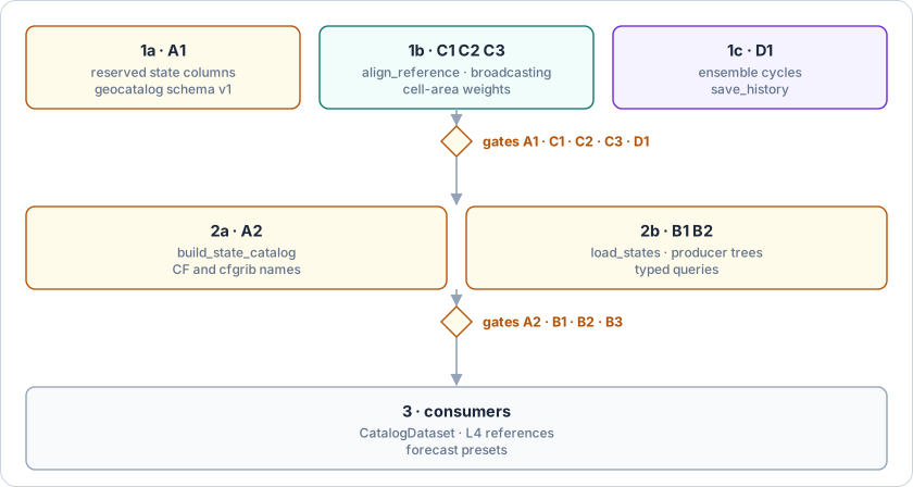
Figure 3:Foundations first, then the state profile, then its consumers.
The first schema migration. A1 is geocatalog’s first registered migration, so a mistake in it touches every saved catalog. Fallback: we ship A2 and B with the four names as documented extra columns and no schema bump, and reserve them once the API has settled.
geocatalog keeps growing. Report 6 found that it had already outgrown its scope. Fallback: if
geocatalog.statespasses about 500 lines, we move it to its own distribution in the geotoolz monorepo, which depends on geocatalog and still has one index format.Metadata conventions vary. CF files, cfgrib-decoded GRIB, and archives that encode the run in the file name all store and differently. Fallback:
namesaccepts a callable on the path, so any archive can be indexed without changing the builder.One row per file is coarse. A file per (run, member) answers “valid at ” at file granularity, so a per-step query must open the file. Fallback: when steps are separate files (common for GRIB), rows are per step without any change, and a per-step explode option is open question 1.
Histories held in memory. A 72-step, 40-member trajectory at 0.25° does not fit in memory. Fallback: we run the cycle in chunks of steps from the last state and write after each chunk, and a streaming hook on the cycles is open question 3.
Pandas query semantics. Users who keep writing
wherestrings still hit stage 2’s silent miss. Fallback: B2’s functions use boolean masks, and thewheredocstring gets a warning about datetime equality.Curvilinear model grids.
regrid_conservativeworks along two rectilinear dimensions, whereas many CMIP ocean models use curvilinear or tripolar native grids (grid_label="gn"). Fallback: we use the regridded products which the modelling centres publish (grid_label="gr"), or regrid those models with an external tool such as xESMF in the script (open question 5).
Open questions
One row per file, or per step? One row per file keeps catalogs small (40 rows for a 40-member run instead of the scoping report’s 2,880), whereas one row per step answers “valid at ” without opening files. Should
build_state_catalogoffer anexplode="step"option?Which kinds?
kindis reserved with three values:analysis,forecast,reanalysis. Do hindcasts and reforecasts need their own values, or are they forecasts with a producer that says so?A streaming hook on the cycles. Should
CycleandEnsembleCycletake anon_step(k, carriers, state)callable, so that scripts can write while the cycle runs? It would also giveSmootherCycleandWindowedCyclea history.Recording assimilated observations. The scoping report’s
states_that_used(obs_slice)needs each analysis to record which observation rows it used. ACatalogBundlematchup table between the analysis and observation catalogs would do it, but is that the right home?Curvilinear grids. Should xrtoolz grow a conservative regrid for curvilinear grids (cell polygons rather than two 1-D weight matrices), or should the stack defer to xESMF for them?
Targets that differ per leaf.
RegridConservativeandRegridLikefix their target grid when built, so regridding one observation field onto each model’s own grid needs one operator per leaf. Should they accept the target as a second input, so the step maps over a tree of targets?
Upcoming work
Table 11 lists the follow-ups.
Table 11:Follow-ups from the reassessment.
| Follow-up | Where | Why |
|---|---|---|
Build CatalogDataset over load_states | pipekit-train | documented in api/datasets.md, not built; it is the emulator-training consumer the scoping report wanted from SimulationDataset |
| Score L4 references from a state catalog | pipekit-evaluate | LEVEL_NAMES["L4"] exists; Task.datasets() could return load_states output as its truth_key |
| Add forecast presets with run and lead dimensions | xrreader (CDS, CMEMS forecast products) | its presets are reanalyses and observations; downloaded forecasts would be indexed with build_state_catalog |
Replace statecatalog in pipekit-train’s design docs | pipekit-train docs/design/architecture.md, api/datasets.md | they list it as a sibling package |
Warn about datetime equality in where | geocatalog InMemoryGeoCatalog.where docstring | stage 2’s silent miss on pandas 3.0.6 |
References
Sources
The scoping report, “Report 13 —
statecatalog: catalog for model states” (supplied by the author).The pinned code in
references/: geocatalog (geotoolz-catalog), xrtoolz and xrreader, pipekit-cycle, pipekit-train, pipekit-experiment and pipekit-evaluate.CF conventions, standard name table (
forecast_reference_time,forecast_period,realization).The running example’s script and outputs, described in Section ??.
- Eyring, V., Bony, S., Meehl, G. A., Senior, C. A., Stevens, B., Stouffer, R. J., & Taylor, K. E. (2016). Overview of the Coupled Model Intercomparison Project Phase 6 (CMIP6) experimental design and organization. Geoscientific Model Development, 9(5), 1937–1958. 10.5194/gmd-9-1937-2016