tracerax: Lagrangian particles and trajectories for JAX
tracerax carries positions forward in time and analyses where they went: particle seeding, deterministic and stochastic advection, binning to grids, footprints, finite-time Lyapunov exponents, residence times and connectivity. It sits at GeoNumerics tier 2, on gridax’s grids, functax’s interpolation and integrix’s stepping, and takes over the particle machinery now inside plumax. Status: proposed, at design-sketch depth.
At a glance
| Layer, tier | GeoNumerics, tier 2 |
| Imports | gridax, geophysix, functax, integrix; JAX, Equinox, diffrax |
| Imported by | plumax; sesmax-ocean (planned); xrops (the planned Lagrangian epic) |
| Takes over | plumax lagrangian: ParticleState, langevin_step, integrate_particles, bin_positions, compute_footprint and the generic loop of simulate_lagrangian |
| Does not own | operators on fields, including semi-Lagrangian advection (finitevolX, spectraldiffx); turbulence closures and source inversions (plumax); velocity at points (functax); time stepping (integrix) |
| Status | proposed; no repository yet |
| Tracked in | the layer map; the companion integrix and gridax designs |
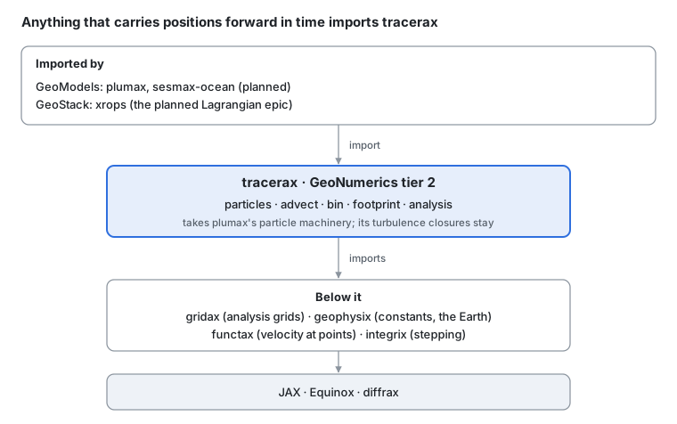
Where tracerax sits · geonumerics tier 2.
The line with finitevolX, settled on the layer map: a scheme that discards its departure points after each step is an operator on a field, and stays with the Eulerian libraries; anything whose state is the positions themselves is tracerax’s. This page is the design; core types, algorithms and the code survey are in tracerax: design details.
The problem
Two questions about a methane plume are Lagrangian. Forward: where does the gas from this source go, and what concentration does it leave in each pixel? Backward: which surface cells could have produced the enhancement this satellite pixel saw? Both release particles, move them with the wind plus turbulence, and count where they end up:
| Step | What it computes | Where it is coded today |
|---|---|---|
| Release and carry particles | a particle state (positions and velocities, all released at t = 0), a Markov-1 Langevin step, and a wind that varies in time only | plumax lagrangian/particles.py: ParticleState, langevin_step, integrate_particles |
| Concentration on a grid | particles binned to cells | plumax lagrangian/concentration.py: bin_positions, simulate_lagrangian |
| Sensitivity of a receptor to surface fluxes | backward integration and residence near the ground | plumax lagrangian/footprint.py: compute_footprint |
| Turbulence for the step | σ_w(z) and τ_L(z) | plumax lagrangian/turbulence.py: HannaTurbulence, HomogeneousTurbulence |
| Transport barriers, retention, connectivity | FTLE, residence time, connectivity matrices | not yet: an empty metrics/_src/lagrangian.py stub in xrops waits for its epic |
The particle machinery is generic, but it sits inside a plume model, so the ocean side (sesmax’s drifters, larval connectivity, retention in eddies) and xrops’ planned Lagrangian views would have to import plumax to use it, or write it again.
Positions carried forward
The state of a Lagrangian calculation is a set of N particles: positions xₚ, masses mₚ, ages, an active flag, and for a stochastic model a velocity fluctuation u’ₚ. Everything in tracerax either moves that state or reads it.
Deterministic advection. Each particle follows the resolved wind, dxₚ/dt = u(xₚ, t), with u at the particle’s position interpolated from a grid by functax and the step taken by an integrix stepper.
Stochastic advection. Unresolved turbulence enters as a Markov-1 Langevin model for the velocity fluctuations: an Ornstein–Uhlenbeck update on all three components, as plumax does it, with the well-mixed drift of Thomson (1987) acting in the vertical, with σ_w(z) the velocity standard deviation and τ_L(z) the Lagrangian time scale supplied by a turbulence closure:
Particles reflect at the ground and, when it is given, at the top of the boundary layer.
Binning. The concentration in cell j of volume Vⱼ is the particle mass inside it:
Footprints. Released backward in time from a receptor, particles that spend time near the ground say how sensitive the receptor is to a surface flux in each cell. With h_s the depth of the surface layer and ρ the air density:
Trajectory analysis. With Φ the flow map that carries a position from t₀ to t₁, the finite-time Lyapunov exponent measures how fast neighbours separate; its ridges are transport barriers:
In JAX the gradient of the flow map is jax.jacfwd of the integration itself, so no finite-difference grid of seeds is needed. Residence time counts how long particles stay in a region; a connectivity matrix Cᵢⱼ counts the fraction released in region i that reaches region j.
Modules and boundaries
Five modules. The particle state is an Equinox module of arrays, so it is a pytree that jax.lax.scan, jit and vmap carry as plumax’s already is.
| Module | Owns | Comes from |
|---|---|---|
tracerax.particles | the particle state; seeding at points, along lines, over regions and over time (plumax releases every particle at t = 0; release over time is new) | plumax ParticleState |
tracerax.advect | deterministic and stochastic advection, in winds that vary in space and time (plumax’s vary in time only, so spatial interpolation through functax is new); the Langevin step; reflection at the ground, the boundary-layer top and coastlines | plumax langevin_step, integrate_particles, n_steps_for_horizon, step_durations |
tracerax.bin | binning to gridax analysis grids or to a model’s own grid: counts, mass, concentration, accumulated residence | plumax bin_positions and the accumulation in simulate_lagrangian |
tracerax.footprint | backward runs from receptors and surface footprints | plumax compute_footprint |
tracerax.analysis | FTLE, residence time, connectivity matrices, dispersion statistics | new; fills the stub in xrops metrics/_src/lagrangian.py |
What tracerax owns, and what it hands off
The test for every name: is its state a set of positions carried forward in time, or does it analyse such positions? Then tracerax owns it.
| Neighbour | tracerax owns | The neighbour owns | The line |
|---|---|---|---|
| finitevolX, spectraldiffx | particles that persist | operators on fields, including semi-Lagrangian advection, which discards its departure points | positions kept from step to step are tracerax’s |
| plumax | the particle machinery | turbulence closures (HannaTurbulence, σ_w(z) and τ_L(z) profiles), plume physics, source inversions | particles take the closure as an argument |
| functax | where the particles go | the wind at a point: interpolation plans | tracerax calls a functax plan for u(xₚ) |
| integrix | the right-hand side and the boundaries | the stepping and its adjoints | an integrix stepper advances the state |
| gridax | binning and the cell a particle is in | analysis grids and their metrics; a model’s grid and masks are finitevolX’s | bins are gridax cells, or finitevolX’s for a model run |
| diagnostix | Lagrangian analysis | Eulerian diagnostics of fields | FTLE is tracerax’s; vorticity is diagnostix’s |
| xrops | the maths | DataArray views of trajectories (the planned Lagrangian epic) | xrops wraps tracerax |
What moves in
| From | What | Its users then import |
|---|---|---|
plumax lagrangian/particles.py | ParticleState, langevin_step, integrate_particles, n_steps_for_horizon, step_durations | tracerax; plumax keeps TurbulenceModel as the protocol its closures satisfy, or tracerax defines it (decision 3) |
plumax lagrangian/concentration.py | bin_positions, the generic loop of simulate_lagrangian | tracerax; plumax keeps a plume-specific simulate_lagrangian built on it |
plumax lagrangian/footprint.py | compute_footprint | tracerax |
| xrops | the empty Lagrangian metrics stub | tracerax.analysis, wrapped by xrops |
In use
The plume both ways: release particles at the source and bin them into a concentration field; release them backward from a satellite pixel and read its surface footprint. Every tracerax name is proposed.
# Shapes: N particles; K steps; Ny × Nx surface cells

import jax
import tracerax as trx
from plumax.lagrangian import HannaTurbulence

release_key, forward_key, backward_key = jax.random.split(jax.random.key(0), 3)


# user
# u(x, t) at particle positions, wrapping a functax interpolation plan
def wind_at(positions, time): ...  # (N, 3) → (N, 3)


# today* (plumax)
# σ_w(z), τ_L(z) from boundary-layer scaling
turbulence = HannaTurbulence(...)

# --- forward: where the gas goes ---
# proposed (tracerax)
particles = trx.particles.release_at(source, n=N, mass=rate * duration, key=release_key)
# proposed (tracerax)
# du' = −u'/τ_L dt + ½ ∂σ_w²/∂z (1 + u'²/σ_w²) dt + (2σ_w²/τ_L)^½ dW
final = trx.advect.langevin(  # (N, 3) → (N, 3)
    particles,
    wind_at,
    turbulence,
    times,
    reflect=trx.advect.Reflect(ground=0.0, top=pbl_height),
    key=forward_key,
)
# proposed (tracerax)
# c_j = ∑ₚ mₚ 1[xₚ ∈ j] / V_j
concentration = trx.bin.concentration(final, grid)  # → (Ny, Nx)

# --- backward: what the pixel could have seen ---
# proposed (tracerax)
# F_j = ∑ₚ ∫ 1[xₚ(t) ∈ j, zₚ(t) < h_s] dt / (N ρ h_s)
footprint = trx.footprint.surface(  # → (Ny, Nx)
    receptor, wind_at, turbulence, grid, duration=600.0, key=backward_key
)
The footprint times a prior flux map is the pixel’s predicted enhancement, which is what an inversion in plumax fits. Because the run is a JAX function, the same footprint is differentiable in the wind and the closure’s parameters.
Integration across the stack
| Consumer | Uses today | With tracerax |
|---|---|---|
| plumax | its own particle state, Langevin step, binning and footprint | tracerax for all four; keeps the turbulence closures, the plume-specific simulation and the inversions |
| sesmax-ocean (planned) | — | drifters, retention in eddies and connectivity on its own velocity fields |
| xrops | an empty Lagrangian stub | DataArray views of trajectories and of tracerax.analysis |
For plumax the change is an import:
# Today:
# today (plumax)
from plumax.lagrangian.particles import ParticleState, langevin_step

# After:
# proposed (tracerax)
from tracerax.particles import ParticleState

# proposed (tracerax)
from tracerax.advect import langevin_step
Decisions and open questions
Three decided, two leaning, two open. Each entry gives the position first, then the trade-off.
1. Layer: GeoNumerics tier 2
Decided (5 Nov 2026, on the layer map). tracerax imports gridax (tier 1), geophysix (tier 0), and functax and integrix (Core). plumax, sesmax-ocean and xrops sit above it.
2. The line with the Eulerian libraries
Decided (5 Nov 2026). A scheme that traces back to departure points and then discards them, such as finitevolX’s semi-Lagrangian advection, is an operator on a field and stays with finitevolX and spectraldiffx. tracerax owns everything whose state is the positions.
3. Turbulence closures stay in plumax
Decided (5 Nov 2026, on the layer map). Particles take σ_w(z) and τ_L(z) through a protocol, and plumax’s closures satisfy it. Open within this: whether tracerax defines the protocol (so that sesmax-ocean can write its own closures without plumax) or plumax keeps it. Leaning: tracerax defines it.
4. Stepping through integrix or a loop of its own
Open. Deterministic advection is an ordinary ODE and fits integrix’s steppers. The Langevin step reflects particles at boundaries, a discrete event that diffrax’s SDE solvers handle awkwardly, and plumax today runs it in a lax.scan of its own. Leaning: deterministic advection through integrix, the stochastic step as tracerax’s own scan with the same adjoint options.
5. Trajectories stored or accumulated
Leaning: accumulate by default. A footprint or a concentration needs only running sums, which plumax already accumulates inside its scan; storing K × N × 3 positions is optional, at chosen times.
6. Randomness
Leaning. One key per run, split once into a key per stage (release, forward, backward) and per step inside the scan, as the house style asks; no global seeds.
7. Coastlines and other boundaries
Open. Reflection at the ground and the boundary-layer top is simple. Reflection at a coastline needs the model’s mask (finitevolX’s Mask2D) and the exact crossing point, which is costly for many particles. Leaning: nearest-wet-cell projection first, exact reflection when an ocean consumer needs it.
Roadmap
Five waves, each a GitHub issue epic in the tracerax repository once it exists.
| Wave | Delivers | Ends | Needs |
|---|---|---|---|
| 0. Scaffold | the repository from the library template; CI, capability index; reference tests against plumax’s Lagrangian outputs | — | gridax wave 1 |
| 1. Particles and advection | tracerax.particles, tracerax.advect | plumax’s particle state and Langevin step | 0; integrix wave 1 |
| 2. Binning and footprints | tracerax.bin, tracerax.footprint | plumax’s binning and footprint | 1 |
| 3. Trajectory analysis | FTLE, residence time, connectivity | the xrops stub | 1 |
| 4. Consumers switch | plumax onto tracerax; xrops’ Lagrangian epic; sesmax-ocean from the start | the copies | 1–3 |
Sources
The GeoStack layer map: tracerax’s layer, tier, imports and moves.
Thomson (1987): the well-mixed condition.
Lin et al. (2003): backward footprints.
Haller (2015): FTLE and transport barriers.
Code read on 5 Nov 2026 at geostack’s submodule pins and xrtoolz
b3855d7: plumaxlagrangian/(particles.py,concentration.py,footprint.py,turbulence.py,inversion.py); xropsmetrics/_src/lagrangian.py; finitevolX’s semi-Lagrangian advection.
- Thomson, D. J. (1987). Criteria for the selection of stochastic models of particle trajectories in turbulent flows. Journal of Fluid Mechanics, 180, 529–556.
- Lin, J. C., Gerbig, C., Wofsy, S. C., Andrews, A. E., Daube, B. C., Davis, K. J., & Grainger, C. A. (2003). A near-field tool for simulating the upstream influence of atmospheric observations: the Stochastic Time-Inverted Lagrangian Transport (STILT) model. Journal of Geophysical Research: Atmospheres, 108(D16), 4493.
- Haller, G. (2015). Lagrangian coherent structures. Annual Review of Fluid Mechanics, 47, 137–162.