Phase 1 — 1D Fundamentals: Advection, Diffusion, and Burgers

The geophysical models later in this book are built from three elementary processes: transport (advection), smoothing (diffusion), and their nonlinear coupling. Each one already contains a numerical lesson that survives all the way up to the shallow-water and quasi-geostrophic models — the CFL limit of explicit advection, the much tighter stability limit of explicit diffusion, and the steepening-versus-smoothing balance that sets the grid Péclet number. This chapter develops the three in one dimension, where the physics is transparent and the somax models run in milliseconds LeVeque (2002)Durran (2010).

What you will learn

Why linear advection on a periodic ring is a pure phase shift, and what the CFL number controls
Why explicit diffusion is limited by $\Delta t \lesssim \Delta x^2 / (2\nu)$ , not $\Delta x$
How the nonlinear Burgers flux steepens a smooth wave into a shock, and how viscosity arrests it

1. Linear advection — transport without distortion¶

The 1-D linear advection equation moves a field $u(x,t)$ at constant speed $c$ without changing its shape,

\partial_t u + c\,\partial_x u = 0,

(1)

with exact solution $u(x,t) = u_0(x - ct)$ — the initial profile translated rigidly. On a periodic domain the solution returns to its start after one transit time $L/c$ . The numerical challenge is that an explicit scheme can only see information within a few cells per step, so the time step is bounded by the Courant–Friedrichs–Lewy (CFL) condition

\mathrm{CFL} \;=\; \frac{c\,\Delta t}{\Delta x} \;\le\; \mathrm{CFL}_{\max},

(2)

where $\mathrm{CFL}_{\max}$ is an $O(1)$ constant set by the time integrator. Above it the scheme is unstable; well below it, numerical diffusion smears the profile. Equation (2) is the one-dimensional ancestor of the gravity-wave CFL that governs every shallow-water run.

import warnings

warnings.filterwarnings("ignore", message=r".*IProgress.*")

import importlib.util
from pathlib import Path

import jax.numpy as jnp
import matplotlib.pyplot as plt

from somax.models import (
    Burgers1D,
    Burgers1DState,
    Diffusion1D,
    Diffusion1DState,
    LinearConvection1D,
    LinearConvection1DState,
)

try:
    from IPython import get_ipython

    ipython = get_ipython()
except ImportError:
    ipython = None

if ipython is not None and importlib.util.find_spec("watermark") is not None:
    ipython.run_line_magic("load_ext", "watermark")
    ipython.run_line_magic("watermark", "-v -m -p numpy,jax,matplotlib,somax")
else:
    print("watermark extension not installed; skipping reproducibility readout.")

watermark extension not installed; skipping reproducibility readout.

IMG_DIR = Path.cwd().parent / "images" / "phase1_fundamentals"
IMG_DIR.mkdir(parents=True, exist_ok=True)

We advect a smooth Gaussian pulse one full transit around a periodic ring. The exact solution returns it to the start; the discrete solution shows the small numerical dispersion/diffusion an explicit upwind scheme introduces over one revolution.

conv = LinearConvection1D.create(nx=200, Lx=1.0, c=1.0)
xc = jnp.linspace(0.0, 1.0, conv.grid.Nx)
pulse0 = jnp.exp(-0.5 * ((xc - 0.3) / 0.05) ** 2)
conv_state0 = conv.apply_boundary_conditions(LinearConvection1DState(u=pulse0))

# One full transit of the periodic domain: t = L / c.
conv_sol = conv.integrate(conv_state0, t0=0.0, t1=1.0, dt=2.0e-3)
pulse_final = conv_sol.ys.u[-1]

cfl = conv.params.c * 2.0e-3 / conv.grid.dx
print(f"advection CFL = {cfl:.3f}")

advection CFL = 0.400

Figure 1 overlays the initial pulse and the field after one full revolution. With the CFL number printed above (well inside the stable range) the pulse returns close to where it started; the slight amplitude loss and broadening is the scheme’s numerical diffusion.

fig, ax = plt.subplots(figsize=(12, 5))
ax.plot(xc, pulse0, "k--", label="initial $u_0(x)$")
ax.plot(xc, pulse_final, "C0", label="after one transit")
ax.set(xlabel="$x$", ylabel="$u$", title="Linear advection on a periodic ring")
ax.legend()
fig.tight_layout()
fig.savefig(IMG_DIR / "advection_transit.png", dpi=110, bbox_inches="tight")
plt.show()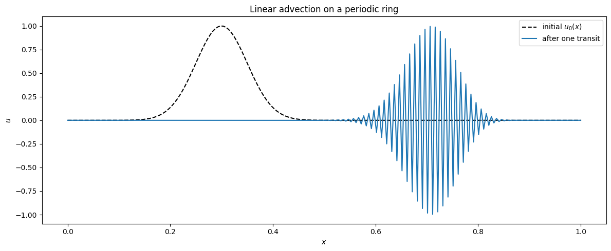

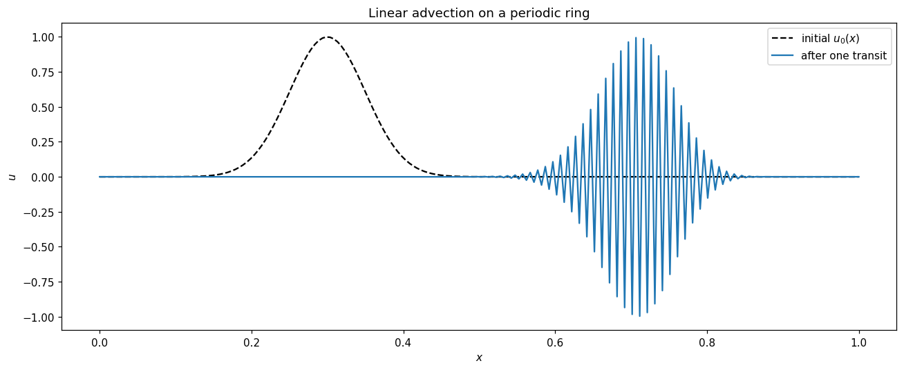
Figure 1:A Gaussian pulse advected one full transit of a periodic domain at unit speed. The dashed curve is the initial condition; the solid curve is the numerical solution after returning to its start. The small broadening is implicit numerical diffusion from the upwind reconstruction.

2. Diffusion — smoothing and the parabolic time-step limit¶

The 1-D diffusion (heat) equation spreads a field at rate set by the diffusivity $\nu$ ,

\partial_t u = \nu\,\partial_{xx} u .

(3)

A Gaussian stays Gaussian, with its variance growing linearly in time, so a blob of initial width $\sigma_0$ has width $\sqrt{\sigma_0^2 + 2\nu t}$ . The crucial numerical fact is that an explicit discretisation of (3) is stable only for

\frac{\nu\,\Delta t}{\Delta x^2} \;\le\; \frac{1}{2},

(4)

a limit that scales with $\Delta x^2$ , not $\Delta x$ . Refining the grid by two therefore demands a four-fold smaller step — the reason stiff diffusion is the term somax tags implicit for IMEX integration (see the composable-models tutorial).

diff_model = Diffusion1D.create(nx=200, Lx=1.0, nu=2.0e-3)
xd = jnp.linspace(0.0, 1.0, diff_model.grid.Nx)
blob0 = jnp.exp(-0.5 * ((xd - 0.5) / 0.04) ** 2)
diff_state0 = diff_model.apply_boundary_conditions(Diffusion1DState(u=blob0))

diff_dt = 5.0e-4
diff_cfl = diff_model.params.nu * diff_dt / diff_model.grid.dx**2
print(f"diffusion number  nu*dt/dx^2 = {diff_cfl:.3f}  (must be <= 0.5)")

snapshots = []
state = diff_state0
for _ in range(4):
    sol = diff_model.integrate(state, t0=0.0, t1=2.0, dt=diff_dt)
    state = Diffusion1DState(u=sol.ys.u[-1])
    snapshots.append(state.u)

diffusion number  nu*dt/dx^2 = 0.040  (must be <= 0.5)

Figure 2 shows the blob broadening and flattening through successive intervals while conserving its integral — the hallmark of a diffusive process.

fig, ax = plt.subplots(figsize=(12, 5))
ax.plot(xd, blob0, "k--", label="$t=0$")
for k, snap in enumerate(snapshots, start=1):
    ax.plot(xd, snap, color=f"C{k - 1}", label=f"$t={2.0 * k:.0f}$")
ax.set(xlabel="$x$", ylabel="$u$", title="1-D diffusion of a Gaussian blob")
ax.legend()
fig.tight_layout()
fig.savefig(IMG_DIR / "diffusion_spread.png", dpi=110, bbox_inches="tight")
plt.show()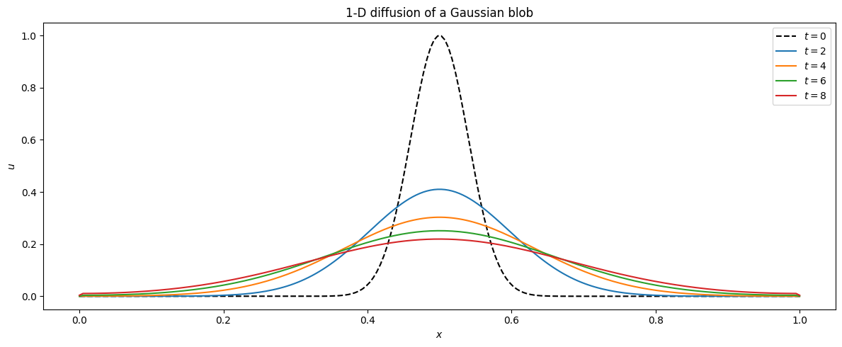

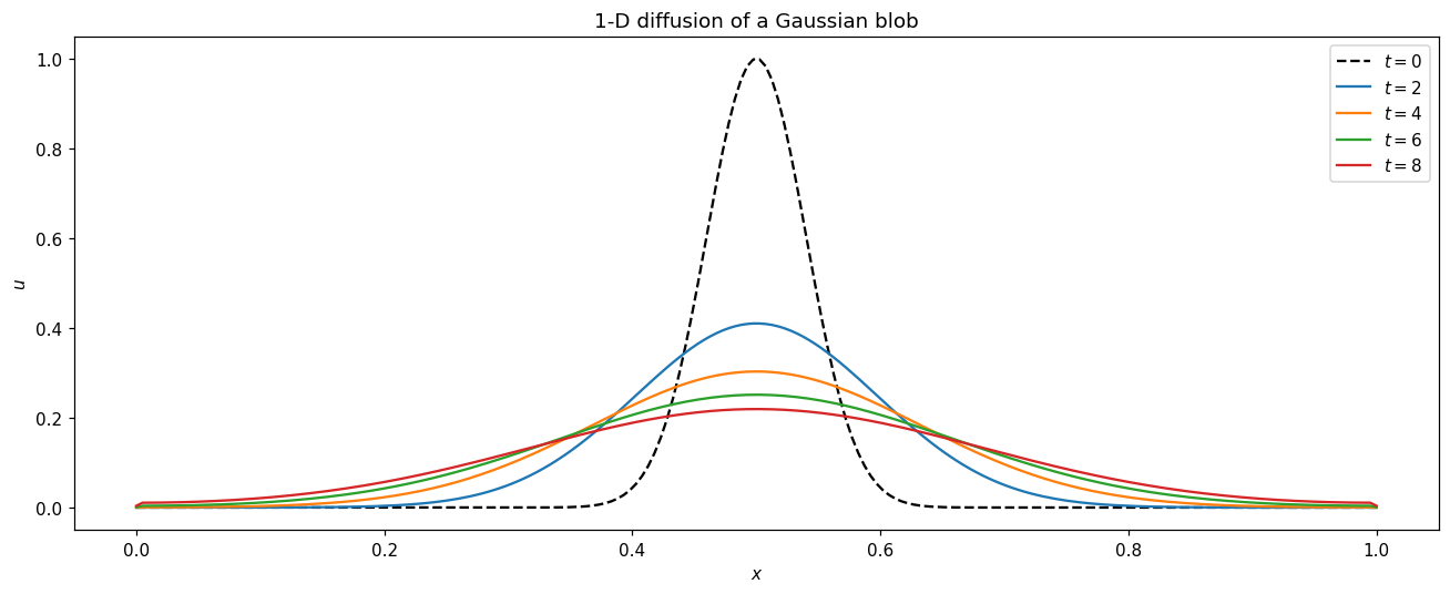
Figure 2:A Gaussian blob diffusing under (3). Each curve is a later time; the peak drops and the profile widens while the area underneath is preserved.

3. Burgers — nonlinear steepening meets viscous smoothing¶

The viscous Burgers equation couples nonlinear self-advection to diffusion,

\partial_t u + u\,\partial_x u = \nu\,\partial_{xx} u ,

(5)

and is the canonical one-dimensional caricature of the Navier–Stokes balance between inertia and viscosity Burgers (1948). Where $u$ is large the wave moves faster, so a smooth profile steepens on its leading edge; the viscous term resists, and the two balance in a thin front of width $\sim \nu / U$ . The relevant dimensionless number is the grid Péclet number $\mathrm{Pe}_{\Delta} = U\,\Delta x / \nu$ : when it exceeds $\sim 2$ the front is under-resolved and the upwind/WENO reconstruction (the operators chapter) controls the spurious oscillations.

burgers = Burgers1D.create(nx=256, Lx=1.0, nu=2.0e-3)
xb = jnp.linspace(0.0, 1.0, burgers.grid.Nx)
sine0 = jnp.sin(2.0 * jnp.pi * xb)
burgers_state0 = burgers.apply_boundary_conditions(Burgers1DState(u=sine0))

burgers_snaps = [sine0]
state = burgers_state0
for _ in range(3):
    sol = burgers.integrate(state, t0=0.0, t1=0.08, dt=5.0e-4)
    state = Burgers1DState(u=sol.ys.u[-1])
    burgers_snaps.append(state.u)

pe_grid = float(jnp.max(jnp.abs(sine0))) * burgers.grid.dx / burgers.params.nu
print(f"grid Peclet number  U*dx/nu = {pe_grid:.2f}")

grid Peclet number  U*dx/nu = 1.95

Figure 3 follows the sine wave as its compressive half steepens toward a near-shock while viscosity keeps the front finite — the steepening/smoothing competition that motivates flux-limited advection schemes.

fig, ax = plt.subplots(figsize=(12, 5))
for k, snap in enumerate(burgers_snaps):
    style = "k--" if k == 0 else f"C{k - 1}"
    ax.plot(xb, snap, style, label=f"$t={0.08 * k:.2f}$")
ax.set(xlabel="$x$", ylabel="$u$", title="Viscous Burgers: steepening vs. smoothing")
ax.legend()
fig.tight_layout()
fig.savefig(IMG_DIR / "burgers_steepening.png", dpi=110, bbox_inches="tight")
plt.show()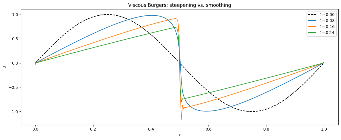

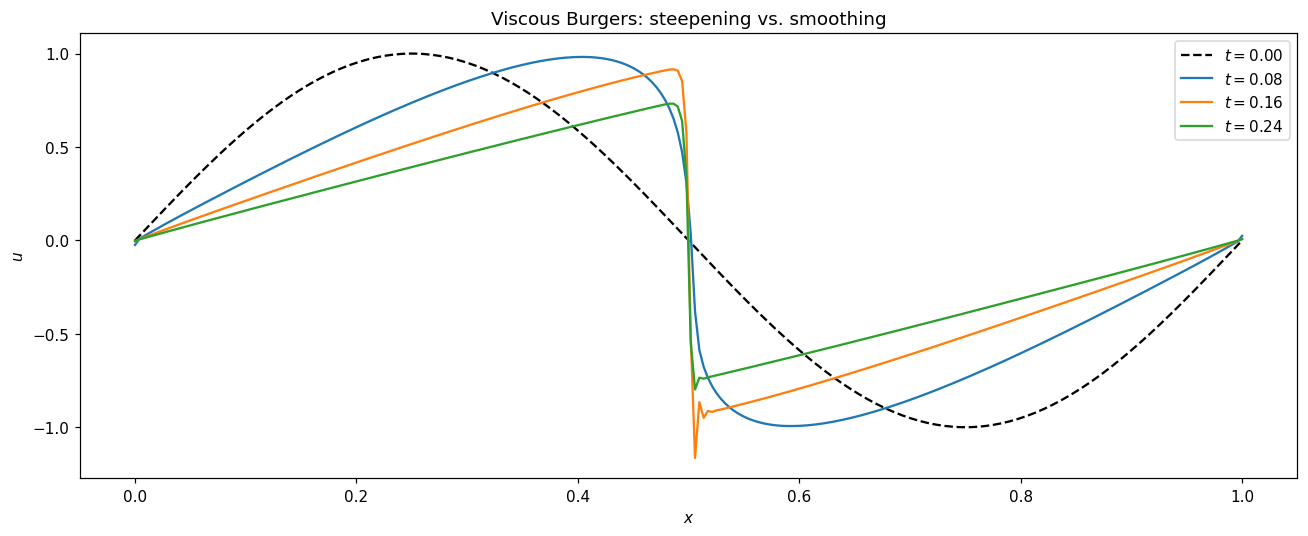
A sine wave evolving under the viscous Burgers equation . The leading edge steepens as the nonlinear flux compresses it; viscosity holds the front at finite width instead of letting it break. — Figure 3:A sine wave evolving under the viscous Burgers equation (5). The leading edge steepens as the nonlinear flux compresses it; viscosity holds the front at finite width instead of letting it break.

Summary¶

The three building blocks and their numerical signatures, gathered in Table 1:

Table 1:The three 1-D processes and the time-step limit each imposes on an explicit scheme.

Process	Equation	Explicit step limit
Advection	(1)	hyperbolic, $c\,\Delta t/\Delta x \le \mathcal{O}(1)$
Diffusion	(3)	parabolic, $\nu\,\Delta t/\Delta x^2 \le 1/2$
Burgers	(5)	both, plus grid-Péclet resolution of the front

Linear advection is a pure translation; the CFL number (2) bounds the explicit step and is the ancestor of the gravity-wave CFL in the shallow-water models.
Explicit diffusion carries the far tighter parabolic limit (4) — the reason somax offers an IMEX path for the stiff Laplacian.
Burgers couples the two: the nonlinear flux steepens, viscosity smooths, and the grid Péclet number decides whether the front is resolved.

The next chapter lifts these processes into two dimensions and adds the elliptic (Poisson) problem that ties velocity to pressure.

References¶

LeVeque, R. J. (2002). Finite Volume Methods for Hyperbolic Problems. Cambridge University Press. 10.1017/CBO9780511791253
Durran, D. R. (2010). Numerical Methods for Fluid Dynamics: With Applications to Geophysics (2nd ed., Vol. 32). Springer. 10.1007/978-1-4419-6412-0
Burgers, J. M. (1948). A mathematical model illustrating the theory of turbulence. Advances in Applied Mechanics, 1, 171–199. 10.1016/S0065-2156(08)70100-5