Phase 2 — 2D Spatial Dynamics: Diffusion, the Poisson Problem, and Cavity Flow

Two dimensions add a qualitatively new ingredient that the 1-D fundamentals could not show: an elliptic constraint. An incompressible flow cannot evolve its vorticity without simultaneously solving a Poisson equation for the streamfunction at every step — a global, instantaneous coupling with no time-step of its own. This chapter builds up to that coupling through 2-D diffusion, the Poisson solve in isolation, and finally the lid-driven cavity, where advection, diffusion, and the elliptic inversion all act together Durran (2010)Cushman-Roisin & Beckers (2011).

What you will learn

How diffusion smooths a 2-D field on the staggered grid
Why incompressible dynamics needs an elliptic (Poisson) solve, and what its solution looks like
How somax’s vorticity–streamfunction Navier–Stokes model assembles advection + diffusion + Poisson into the canonical cavity benchmark

1. Two-dimensional diffusion¶

The 2-D diffusion equation smooths a field isotropically,

\partial_t u = \nu\,\nabla^2 u = \nu\left(\partial_{xx} u + \partial_{yy} u\right),

(1)

and inherits the parabolic step limit from one dimension in a slightly stricter form, $\nu\,\Delta t\,(\Delta x^{-2} + \Delta y^{-2}) \le 1/2$ . A compact blob relaxes into an ever-wider, ever-flatter mound while conserving its integral — the multidimensional version of the smoothing seen in (1).

import warnings

warnings.filterwarnings("ignore", message=r".*IProgress.*")

import importlib.util
from pathlib import Path

import jax.numpy as jnp
import matplotlib.pyplot as plt

from somax.models import (
    Diffusion2D,
    Diffusion2DState,
    IncompressibleNS2D,
    NSVorticityState,
    PoissonSolver2D,
)

try:
    from IPython import get_ipython

    ipython = get_ipython()
except ImportError:
    ipython = None

if ipython is not None and importlib.util.find_spec("watermark") is not None:
    ipython.run_line_magic("load_ext", "watermark")
    ipython.run_line_magic("watermark", "-v -m -p numpy,jax,matplotlib,somax")
else:
    print("watermark extension not installed; skipping reproducibility readout.")

watermark extension not installed; skipping reproducibility readout.

IMG_DIR = Path.cwd().parent / "images" / "phase2_spatial"
IMG_DIR.mkdir(parents=True, exist_ok=True)

diff2d = Diffusion2D.create(nx=96, ny=96, Lx=1.0, Ly=1.0, nu=2.0e-3)
xd = jnp.linspace(0.0, 1.0, diff2d.grid.Nx)
yd = jnp.linspace(0.0, 1.0, diff2d.grid.Ny)
Xd, Yd = jnp.meshgrid(xd, yd)
blob0 = jnp.exp(-0.5 * (((Xd - 0.5) / 0.05) ** 2 + ((Yd - 0.5) / 0.05) ** 2))
diff_state0 = diff2d.apply_boundary_conditions(Diffusion2DState(u=blob0))

diff_sol = diff2d.integrate(diff_state0, t0=0.0, t1=8.0, dt=2.0e-3, max_steps=20000)
blob_final = diff_sol.ys.u[-1]

Figure 1 contrasts the initial spike with the relaxed field.

fig, axes = plt.subplots(1, 2, figsize=(12, 5))
for ax, field, ttl in zip(axes, [blob0, blob_final], ["$t=0$", "$t=8$"], strict=True):
    im = ax.pcolormesh(Xd, Yd, field, cmap="magma", vmin=0.0, vmax=1.0)
    ax.set(xlabel="$x$", ylabel="$y$", title=ttl, aspect="equal")
    fig.colorbar(im, ax=ax, shrink=0.8)
fig.suptitle("2-D diffusion of a Gaussian blob")
fig.tight_layout()
fig.savefig(IMG_DIR / "diffusion2d.png", dpi=110, bbox_inches="tight")
plt.show()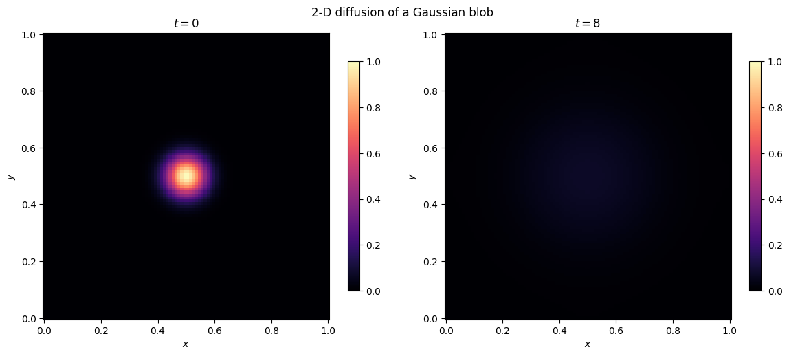

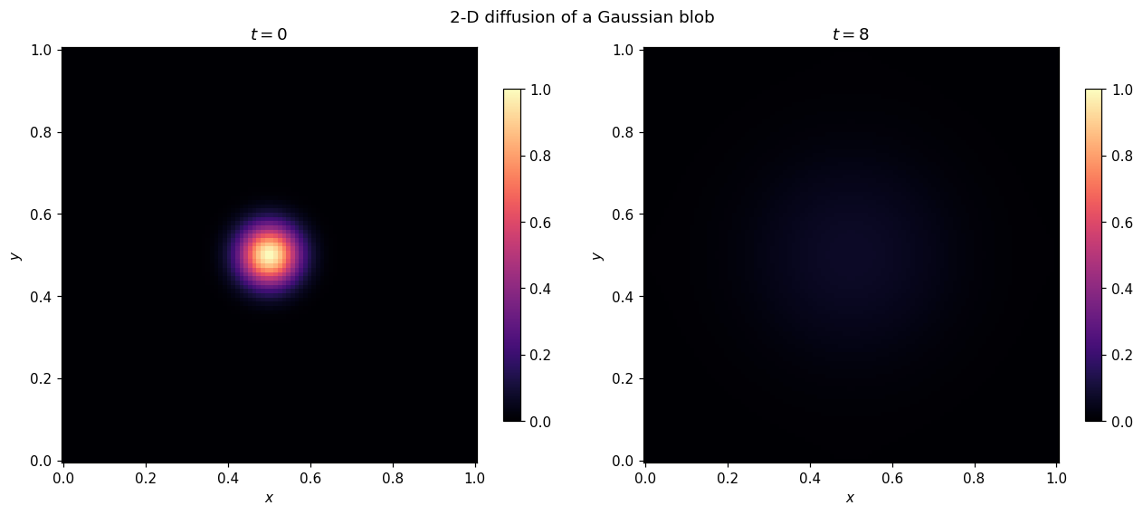
A 2-D Gaussian blob before and after diffusing under . The peak collapses and the support broadens isotropically. — Figure 1:A 2-D Gaussian blob before and after diffusing under (1). The peak collapses and the support broadens isotropically.

2. The Poisson problem — the elliptic heart of incompressible flow¶

An incompressible 2-D flow is divergence-free, so it derives from a streamfunction $\psi$ with $\mathbf{u} = (-\partial_y\psi,\ \partial_x\psi)$ . Its vorticity $\omega = \partial_x v - \partial_y u$ then satisfies a Poisson equation,

\nabla^2 \psi = \omega ,

(2)

which must be solved — globally and instantaneously — to recover the velocity from the vorticity at every time step. Unlike advection or diffusion, (2) has no time derivative: it is an elliptic constraint, and its fast, accurate inversion is the workhorse behind both the Navier–Stokes cavity below and the quasi-geostrophic models of Phase 4. somax exposes the inversion directly as PoissonSolver2D.

poisson = PoissonSolver2D.create(nx=128, ny=128, Lx=1.0, Ly=1.0, bc="dirichlet")
xp = jnp.linspace(0.0, 1.0, poisson.grid.Nx)
yp = jnp.linspace(0.0, 1.0, poisson.grid.Ny)
Xp, Yp = jnp.meshgrid(xp, yp)

# A localized vorticity source: a positive and a negative blob (a vortex pair).
omega_src = jnp.exp(-((Xp - 0.35) ** 2 + (Yp - 0.5) ** 2) / 0.01) - jnp.exp(
    -((Xp - 0.65) ** 2 + (Yp - 0.5) ** 2) / 0.01
)
psi = poisson.solve(omega_src)
print(
    f"Poisson solve: psi shape {psi.shape}, finite={bool(jnp.all(jnp.isfinite(psi)))}"
)

Poisson solve: psi shape (130, 130), finite=True

Figure 2 shows the source on the left and the recovered streamfunction on the right; the closed $\psi$ contours are the streamlines of the vortex pair that the source implies.

fig, axes = plt.subplots(1, 2, figsize=(12, 5))
im0 = axes[0].pcolormesh(Xp, Yp, omega_src, cmap="RdBu_r")
axes[0].set(xlabel="$x$", ylabel="$y$", title=r"source $\omega$", aspect="equal")
fig.colorbar(im0, ax=axes[0], shrink=0.8)
im1 = axes[1].pcolormesh(Xp, Yp, psi, cmap="viridis")
axes[1].contour(Xp, Yp, psi, levels=12, colors="k", alpha=0.4, linewidths=0.6)
axes[1].set(xlabel="$x$", ylabel="$y$", title=r"streamfunction $\psi$", aspect="equal")
fig.colorbar(im1, ax=axes[1], shrink=0.8)
fig.suptitle(r"Poisson inversion $\nabla^2\psi=\omega$")
fig.tight_layout()
fig.savefig(IMG_DIR / "poisson.png", dpi=110, bbox_inches="tight")
plt.show()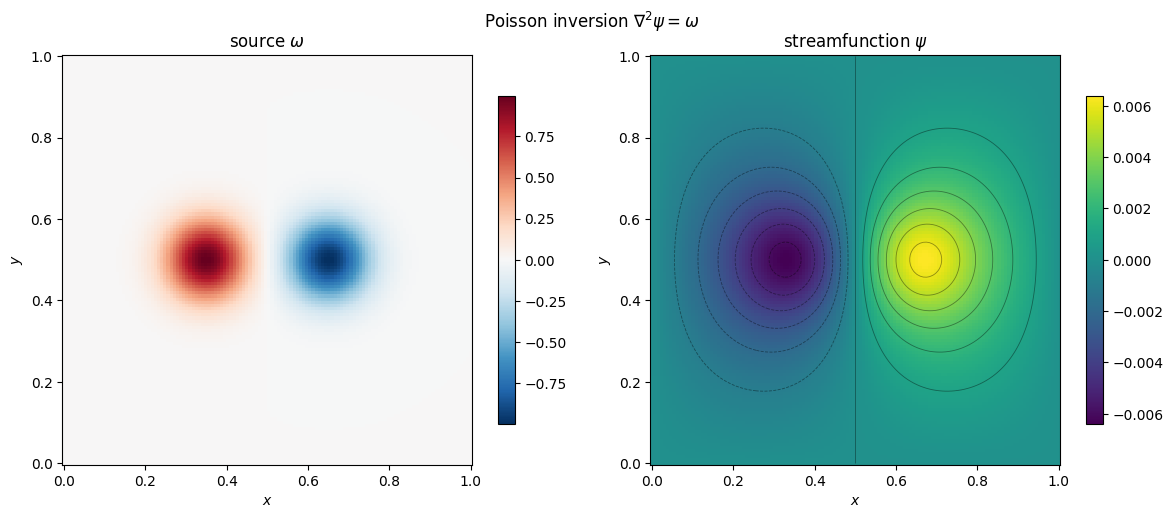

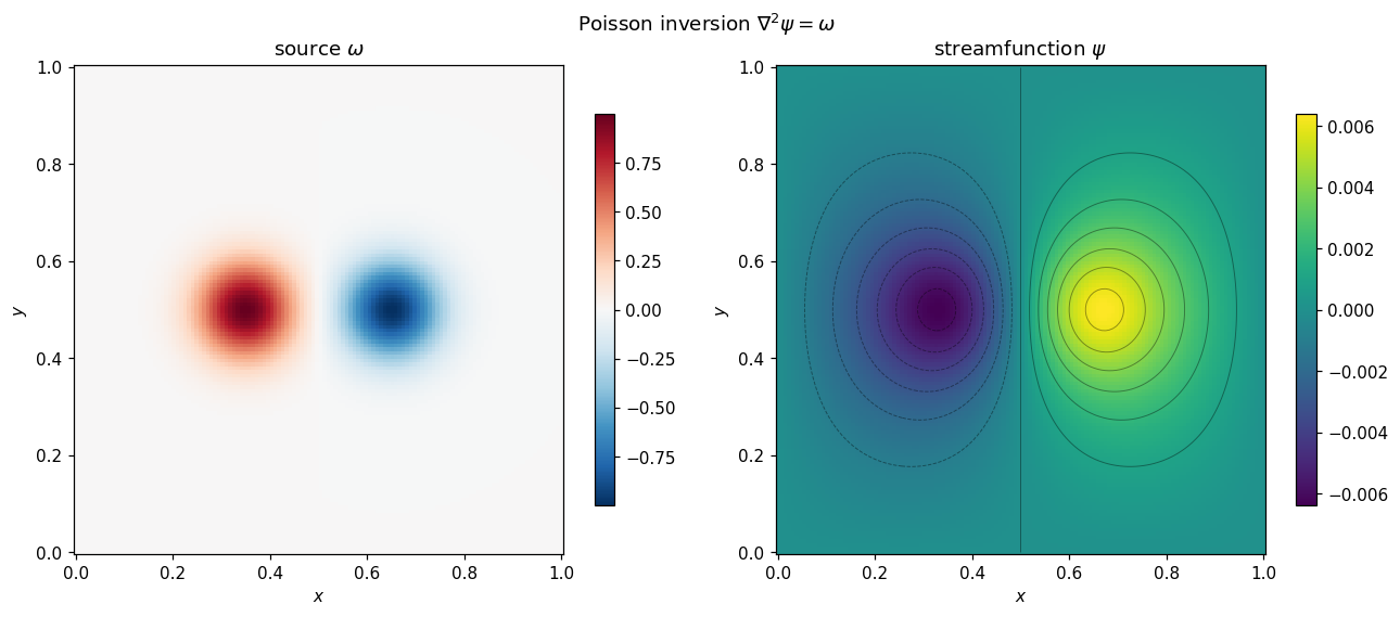
Left: a dipolar vorticity source. Right: the streamfunction recovered by inverting with homogeneous Dirichlet boundaries; the contours are the implied streamlines. — Figure 2:Left: a dipolar vorticity source. Right: the streamfunction recovered by inverting (2) with homogeneous Dirichlet boundaries; the contours are the implied streamlines.

3. Lid-driven cavity — advection, diffusion, and Poisson together¶

The lid-driven cavity is the standard benchmark that exercises all three ingredients at once. The vorticity transport equation

\partial_t \omega + \mathbf{u}\cdot\nabla\omega = \nu\,\nabla^2\omega , \qquad \nabla^2\psi = \omega ,

(3)

is integrated in a square box whose top wall slides at constant speed while the other three are no-slip. Vorticity is generated at the moving lid, advected into the interior, diffused, and continuously re-inverted through (3) to update the velocity. somax’s IncompressibleNS2D assembles exactly this loop.

cavity = IncompressibleNS2D.create(
    nx=96, ny=96, Lx=1.0, Ly=1.0, nu=2.0e-3, problem="cavity", u_lid=1.0
)
cav_state0 = cavity.apply_boundary_conditions(
    NSVorticityState(omega=jnp.zeros((cavity.grid.Ny, cavity.grid.Nx)))
)
cav_sol = cavity.integrate(cav_state0, t0=0.0, t1=5.0, dt=2.5e-3, max_steps=20000)
omega_final = cav_sol.ys.omega[-1]
psi_final = cavity._solve_psi(omega_final)
print(f"cavity Reynolds number ~ u_lid*L/nu = {1.0 * 1.0 / 2.0e-3:.0f}")

cavity Reynolds number ~ u_lid*L/nu = 500

Figure 3 shows the spun-up cavity: the primary recirculating vortex fills the box, driven by the lid, with the streamfunction contours revealing the characteristic central eddy and weaker bottom-corner circulations.

xc = jnp.linspace(0.0, 1.0, cavity.grid.Nx)
yc = jnp.linspace(0.0, 1.0, cavity.grid.Ny)
Xc, Yc = jnp.meshgrid(xc, yc)
fig, axes = plt.subplots(1, 2, figsize=(12, 5))
im0 = axes[0].pcolormesh(Xc, Yc, omega_final, cmap="RdBu_r")
axes[0].set(xlabel="$x$", ylabel="$y$", title=r"vorticity $\omega$", aspect="equal")
fig.colorbar(im0, ax=axes[0], shrink=0.8)
axes[1].contour(Xc, Yc, psi_final, levels=20, colors="C0", linewidths=0.7)
axes[1].set(xlabel="$x$", ylabel="$y$", title=r"streamlines $\psi$", aspect="equal")
fig.suptitle("Lid-driven cavity (lid slides along the top)")
fig.tight_layout()
fig.savefig(IMG_DIR / "cavity.png", dpi=110, bbox_inches="tight")
plt.show()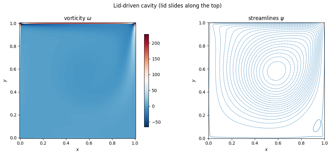

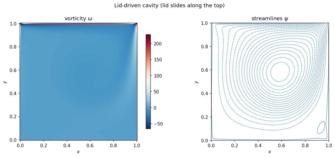
Lid-driven cavity at moderate Reynolds number. Left: vorticity, generated at the sliding top wall and swept around the box. Right: streamlines from the Poisson inversion , showing the primary central vortex. — Figure 3:Lid-driven cavity at moderate Reynolds number. Left: vorticity, generated at the sliding top wall and swept around the box. Right: streamlines from the Poisson inversion (3), showing the primary central vortex.

Summary¶

2-D diffusion (1) smooths isotropically under a parabolic step limit, the direct extension of the 1-D case.
Incompressible flow carries an elliptic constraint: the Poisson equation (2) must be inverted every step to recover velocity from vorticity — a global coupling with no time-step of its own, exposed as PoissonSolver2D.
The lid-driven cavity (3) welds advection, diffusion, and the Poisson solve into one loop; the same vorticity–streamfunction structure reappears in the quasi-geostrophic ocean models.

With the elliptic machinery in place, the next chapter turns to low-order chaos — the Lorenz systems — before Phase 4 assembles the full geophysical models.

References¶

Durran, D. R. (2010). Numerical Methods for Fluid Dynamics: With Applications to Geophysics (2nd ed., Vol. 32). Springer. 10.1007/978-1-4419-6412-0
Cushman-Roisin, B., & Beckers, J.-M. (2011). Introduction to Geophysical Fluid Dynamics: Physical and Numerical Aspects (2nd ed., Vol. 101). Academic Press.