Phase 3 — Chaos and Predictability: the Lorenz Systems

Before tackling the full fluid models, it is worth meeting deterministic chaos in its smallest form. Edward Lorenz’s two systems — a three-variable convection caricature and an $N$ -variable atmospheric ring — distil the property that makes weather and ocean forecasting hard: a perfectly known, perfectly deterministic system whose trajectories nonetheless become unpredictable because minuscule differences in the initial state grow exponentially Lorenz (1963)Lorenz (1996). somax ships both as first-class models, and they are the standard test-beds for the data-assimilation machinery in later tutorials.

What you will learn

How the Lorenz-63 system traces out its butterfly attractor
What “sensitive dependence on initial conditions” looks like quantitatively
How the Lorenz-96 ring produces travelling spatiotemporal chaos

1. Lorenz-63 — the butterfly attractor¶

The Lorenz-63 system is three coupled ODEs distilled from Rayleigh–Bénard convection,

\begin{aligned} \dot{x} &= \sigma\,(y - x), \\ \dot{y} &= x\,(\rho - z) - y, \\ \dot{z} &= x\,y - \beta\,z, \end{aligned}

(1)

with the classical parameters $(\sigma,\rho,\beta) = (10,\ 28,\ 8/3)$ at which the flow is chaotic Lorenz (1963). Trajectories are drawn onto a bounded, fractal strange attractor — the two-lobed “butterfly” — never repeating yet never escaping.

import warnings

warnings.filterwarnings("ignore", message=r".*IProgress.*")

import importlib.util
from pathlib import Path

import diffrax as dfx
import jax.numpy as jnp
import matplotlib.pyplot as plt

from somax.models import Lorenz63, Lorenz96, L63State, L96State

try:
    from IPython import get_ipython

    ipython = get_ipython()
except ImportError:
    ipython = None

if ipython is not None and importlib.util.find_spec("watermark") is not None:
    ipython.run_line_magic("load_ext", "watermark")
    ipython.run_line_magic("watermark", "-v -m -p numpy,jax,matplotlib,somax")
else:
    print("watermark extension not installed; skipping reproducibility readout.")

watermark extension not installed; skipping reproducibility readout.

IMG_DIR = Path.cwd().parent / "images" / "phase3_chaos"
IMG_DIR.mkdir(parents=True, exist_ok=True)

l63 = Lorenz63.create(sigma=10.0, rho=28.0, beta=8.0 / 3.0)
state0 = L63State(x=jnp.array(1.0), y=jnp.array(1.0), z=jnp.array(1.0))

ts = jnp.arange(0.0, 50.0, 0.01)
sol = l63.integrate(
    state0, t0=0.0, t1=50.0, dt=0.01, saveat=dfx.SaveAt(ts=ts), max_steps=20000
)
print(f"L63 trajectory: {sol.ys.x.shape[0]} samples")

L63 trajectory: 5000 samples

Figure 1 projects the trajectory onto the $(x,z)$ plane, tracing the two wings of the attractor between which the state irregularly switches.

fig, ax = plt.subplots(figsize=(12, 5))
ax.plot(sol.ys.x, sol.ys.z, color="C0", lw=0.4)
ax.set(xlabel="$x$", ylabel="$z$", title="Lorenz-63 attractor ($x$-$z$ projection)")
fig.tight_layout()
fig.savefig(IMG_DIR / "l63_attractor.png", dpi=110, bbox_inches="tight")
plt.show()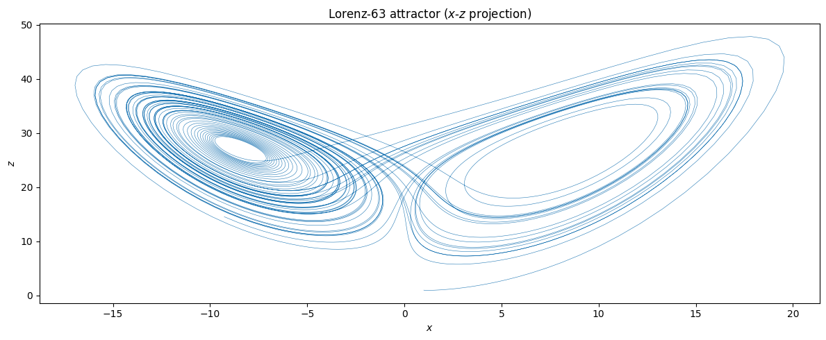

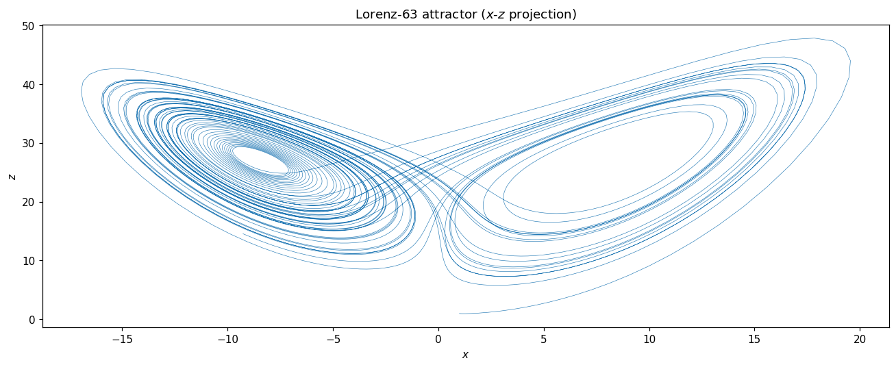
The Lorenz-63 strange attractor , projected onto the (x,z) plane. The trajectory winds around two lobes, switching between them aperiodically — the signature of low-dimensional chaos. — Figure 1:The Lorenz-63 strange attractor (1), projected onto the $(x,z)$ plane. The trajectory winds around two lobes, switching between them aperiodically — the signature of low-dimensional chaos.

2. Sensitive dependence on initial conditions¶

Chaos is quantified by the exponential separation of nearby trajectories. Two states that start a tiny distance $\delta_0$ apart diverge, on average, as

\delta(t) \;\sim\; \delta_0\,e^{\lambda t},

(2)

where $\lambda > 0$ is the leading Lyapunov exponent ( $\lambda \approx 0.9$ for Lorenz-63). The finite growth horizon this implies — not any model deficiency — is the fundamental limit on forecast skill Lorenz (1963). We integrate two trajectories whose initial conditions differ by 10^-6 and watch the gap. (We use 10^-6 rather than a smaller value because somax runs in single precision by default, where perturbations below $\sim\!10^{-7}$ vanish into round-off.)

pert = 1.0e-6
state_a = L63State(x=jnp.array(1.0), y=jnp.array(1.0), z=jnp.array(1.0))
state_b = L63State(x=jnp.array(1.0 + pert), y=jnp.array(1.0), z=jnp.array(1.0))

ts2 = jnp.arange(0.0, 40.0, 0.01)
sol_a = l63.integrate(
    state_a, t0=0.0, t1=40.0, dt=0.01, saveat=dfx.SaveAt(ts=ts2), max_steps=20000
)
sol_b = l63.integrate(
    state_b, t0=0.0, t1=40.0, dt=0.01, saveat=dfx.SaveAt(ts=ts2), max_steps=20000
)

sep = jnp.sqrt(
    (sol_a.ys.x - sol_b.ys.x) ** 2
    + (sol_a.ys.y - sol_b.ys.y) ** 2
    + (sol_a.ys.z - sol_b.ys.z) ** 2
)
print(f"initial separation {pert:.0e} → final separation {float(sep[-1]):.2f}")

initial separation 1e-06 → final separation 17.68

Figure 2 plots the separation on a log axis. The early near-straight ramp is the exponential growth of (2); its slope is the leading Lyapunov exponent. Growth saturates once the gap reaches the size of the attractor itself — at which point the two forecasts are effectively independent.

fig, ax = plt.subplots(figsize=(12, 5))
ax.semilogy(ts2, sep, color="C1")
ax.set(
    xlabel="time",
    ylabel=r"separation $\delta(t)$",
    title="Sensitive dependence: two trajectories $10^{-6}$ apart",
)
fig.tight_layout()
fig.savefig(IMG_DIR / "l63_divergence.png", dpi=110, bbox_inches="tight")
plt.show()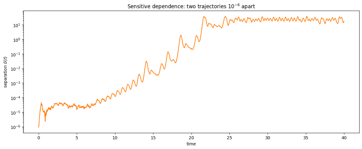

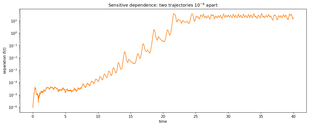
Separation between two Lorenz-63 trajectories whose initial states differ by 10^{-6}. The log-linear ramp is the exponential divergence ; saturation occurs when the separation reaches the attractor’s own scale. — Figure 2:Separation between two Lorenz-63 trajectories whose initial states differ by 10^-6. The log-linear ramp is the exponential divergence (2); saturation occurs when the separation reaches the attractor’s own scale.

3. Lorenz-96 — spatiotemporal chaos on a ring¶

Lorenz-96 extends the idea to $K$ variables arranged on a periodic ring, each representing an atmospheric quantity at one longitude,

\dot{x}_k = (x_{k+1} - x_{k-2})\,x_{k-1} - x_k + F, \qquad k = 1,\dots,K,

(3)

with cyclic indices and a constant forcing $F$ Lorenz (1996). The quadratic term advects, the linear term damps, and $F$ injects energy; at $F=8$ the balance produces travelling waves that break into sustained spatiotemporal chaos. Because it is high-dimensional yet cheap, Lorenz-96 is the standard proving ground for data-assimilation schemes.

l96 = Lorenz96.create(F=8.0)
state96 = L96State.init_state(ndim=40, noise=0.01, F=8.0)

ts96 = jnp.arange(0.0, 20.0, 0.01)
sol96 = l96.integrate(
    state96, t0=0.0, t1=20.0, dt=0.01, saveat=dfx.SaveAt(ts=ts96), max_steps=20000
)
hovmoller = sol96.ys.x
print(f"L96 Hovmoller: {hovmoller.shape} (time, longitude)")

L96 Hovmoller: (2000, 40) (time, longitude)

Figure 3 is a Hovmöller diagram — longitude on the horizontal axis, time on the vertical — of the 40-variable ring. The slanted bands are westward-propagating waves; their irregular merging and splitting is the spatiotemporal chaos that makes the system a faithful, low-cost atmosphere surrogate.

fig, ax = plt.subplots(figsize=(12, 5))
im = ax.pcolormesh(jnp.arange(40), ts96, hovmoller, cmap="RdBu_r", shading="auto")
ax.set(xlabel="longitude index $k$", ylabel="time", title="Lorenz-96 Hovmöller ($F=8$)")
fig.colorbar(im, ax=ax, shrink=0.8, label="$x_k$")
fig.tight_layout()
fig.savefig(IMG_DIR / "l96_hovmoller.png", dpi=110, bbox_inches="tight")
plt.show()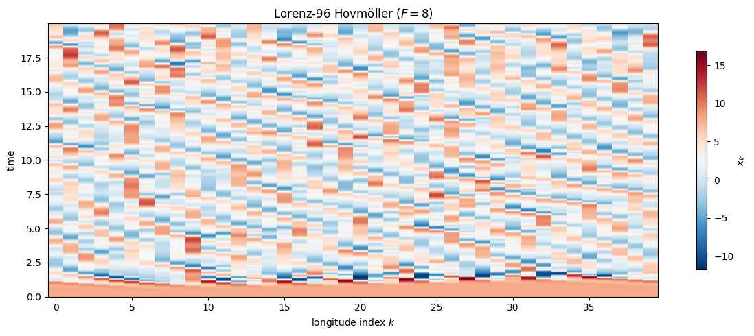

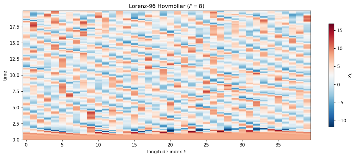
Hovmöller diagram of the Lorenz-96 ring at F=8. Slanted stripes are propagating waves; their continual reorganisation is sustained spatiotemporal chaos. — Figure 3:Hovmöller diagram of the Lorenz-96 ring (3) at $F=8$ . Slanted stripes are propagating waves; their continual reorganisation is sustained spatiotemporal chaos.

Summary¶

Lorenz-63 (1) traces a bounded strange attractor; the flow is deterministic yet never repeats.
Sensitive dependence — exponential separation (2) of nearby states at the positive Lyapunov rate — is the intrinsic limit on predictability, not a numerical artifact.
Lorenz-96 (3) lifts chaos onto a ring, giving high-dimensional spatiotemporal chaos at trivial cost — the canonical data-assimilation test-bed used in the ETKF and 4DVar tutorials.

The final chapter brings the staggered grids, operators, and elliptic solvers of Phases 0–2 together into the geophysical shallow-water and quasi-geostrophic models.

References¶

Lorenz, E. N. (1963). Deterministic nonperiodic flow. Journal of the Atmospheric Sciences, 20(2), 130–141. https://doi.org/10.1175/1520-0469(1963)020<;0130:DNF>2.0.CO;2
Lorenz, E. N. (1996). Predictability: A problem partly solved. Proceedings of the Seminar on Predictability, 1, 1–18.