Phase 4 — Geophysical Fluid Dynamics: Shallow Water and Quasi-Geostrophy

This final chapter assembles everything from the earlier phases — the staggered grid, the discrete operators, the elliptic solver — into the two model families at the heart of somax: the rotating shallow-water equations and their slow-manifold reduction, the quasi-geostrophic equations. Rotation is the new physics: it introduces the Coriolis force, geostrophic balance, the deformation radius, and the westward-propagating Rossby waves that organise the ocean’s large-scale circulation Vallis (2017)Cushman-Roisin & Beckers (2011)Pedlosky (1987).

What you will learn

How a free-surface bump adjusts toward geostrophic balance, radiating gravity waves
What geostrophic balance means for the velocity and height fields
How a quasi-geostrophic flow conserves potential vorticity while shedding Rossby waves

1. The rotating shallow-water equations¶

The single-layer rotating shallow-water equations evolve a height field $h$ and horizontal velocity $\mathbf{u}=(u,v)$ on an $f$ -plane,

\partial_t \mathbf{u} + (\mathbf{u}\cdot\nabla)\mathbf{u} + f\,\hat{\mathbf{z}}\times\mathbf{u} = -g\,\nabla h ,

(1)

\partial_t h + \nabla\cdot(h\,\mathbf{u}) = 0 ,

(2)

where $f$ is the Coriolis parameter and $g$ gravity. The Coriolis term $f\,\hat{\mathbf{z}}\times\mathbf{u}$ turns moving fluid to the right (northern hemisphere) and is what distinguishes geophysical flow from the cavity flow of Phase 2. The fastest signal is the external gravity wave with speed $c=\sqrt{gH}$ , which sets the CFL limit for an explicit run.

import warnings

warnings.filterwarnings("ignore", message=r".*IProgress.*")

import importlib.util
from pathlib import Path

import jax.numpy as jnp
import matplotlib.pyplot as plt

from somax.models import (
    BarotropicQG,
    BarotropicQGState,
    NonlinearShallowWater2D,
    NonlinearSW2DState,
)

try:
    from IPython import get_ipython

    ipython = get_ipython()
except ImportError:
    ipython = None

if ipython is not None and importlib.util.find_spec("watermark") is not None:
    ipython.run_line_magic("load_ext", "watermark")
    ipython.run_line_magic("watermark", "-v -m -p numpy,jax,matplotlib,somax")
else:
    print("watermark extension not installed; skipping reproducibility readout.")

watermark extension not installed; skipping reproducibility readout.

IMG_DIR = Path.cwd().parent / "images" / "phase4_gfd"
IMG_DIR.mkdir(parents=True, exist_ok=True)

2. Geostrophic adjustment¶

Release a mound of fluid in a rotating system and it does not simply collapse. Rotation arrests the spreading: the flow accelerates down the pressure gradient, is deflected by Coriolis, and settles into a balance in which the pressure gradient is held up by the Coriolis force — geostrophic balance,

f\,u = -g\,\partial_y h, \qquad f\,v = g\,\partial_x h .

(3)

The excess height that cannot be balanced is radiated away as gravity waves, leaving a balanced vortex behind. The horizontal scale over which adjustment happens is the Rossby radius of deformation $L_d = \sqrt{gH}/f$ . We initialise a Gaussian sea-surface-height bump at rest and integrate.

swm = NonlinearShallowWater2D.create(
    nx=96,
    ny=96,
    Lx=2e6,
    Ly=2e6,
    f0=1e-4,
    H0=1000.0,
    lateral_viscosity=50.0,
    bc="periodic",
)
xs = jnp.arange(swm.grid.Nx) * swm.grid.dx
ys = jnp.arange(swm.grid.Ny) * swm.grid.dy
Xs, Ys = jnp.meshgrid(xs, ys)
bump = 2.0 * jnp.exp(-(((Xs - 1e6) ** 2 + (Ys - 1e6) ** 2) / (2e5) ** 2))
swm_state0 = NonlinearSW2DState(
    h=swm.consts.H0 + bump, u=jnp.zeros_like(bump), v=jnp.zeros_like(bump)
)

# Gravity-wave CFL: c = sqrt(g H0); keep dt so c*dt/dx < 1/2.
c_ext = jnp.sqrt(9.81 * swm.consts.H0)
dx_min = min(swm.grid.dx, swm.grid.dy)
print(f"external wave speed sqrt(gH) = {float(c_ext):.0f} m/s, dx = {dx_min:.0f} m")
Ld = float(c_ext) / swm.consts.f0
print(f"deformation radius L_d = sqrt(gH)/f = {Ld / 1e3:.0f} km")

swm_sol = swm.integrate(swm_state0, t0=0.0, t1=2 * 86400.0, dt=100.0, max_steps=40000)
h_final = swm_sol.ys.h[-1]
diag_final = swm.diagnose(
    NonlinearSW2DState(h=h_final, u=swm_sol.ys.u[-1], v=swm_sol.ys.v[-1])
)

external wave speed sqrt(gH) = 99 m/s, dx = 20833 m
deformation radius L_d = sqrt(gH)/f = 990 km

Figure 1 compares the initial height anomaly with the field after two days. The central bump has partially slumped and is now encircled by a balanced geostrophic flow (shown as the velocity vorticity), with concentric gravity-wave fronts radiating outward through the periodic domain.

fig, axes = plt.subplots(1, 2, figsize=(12, 5))
im0 = axes[0].pcolormesh(Xs / 1e3, Ys / 1e3, bump, cmap="magma", shading="auto")
axes[0].set(
    xlabel="x (km)", ylabel="y (km)", title="initial SSH anomaly", aspect="equal"
)
fig.colorbar(im0, ax=axes[0], shrink=0.8, label="m")
im1 = axes[1].pcolormesh(
    Xs / 1e3,
    Ys / 1e3,
    diag_final.relative_vorticity,
    cmap="RdBu_r",
    shading="auto",
)
axes[1].set(
    xlabel="x (km)", ylabel="y (km)", title="vorticity after 2 days", aspect="equal"
)
fig.colorbar(im1, ax=axes[1], shrink=0.8, label="s$^{-1}$")
fig.suptitle("Geostrophic adjustment of a height anomaly")
fig.tight_layout()
fig.savefig(IMG_DIR / "geostrophic_adjustment.png", dpi=110, bbox_inches="tight")
plt.show()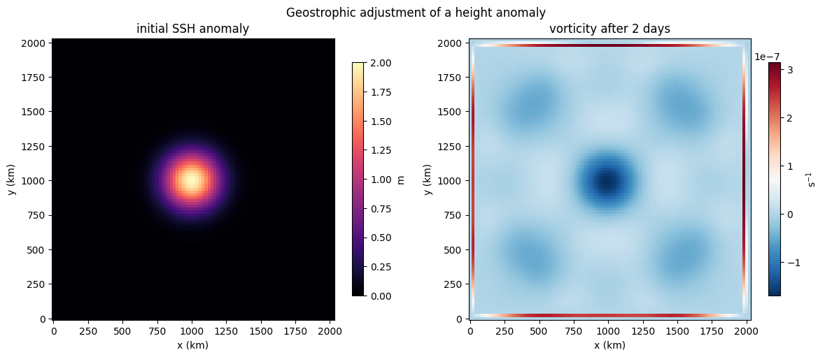

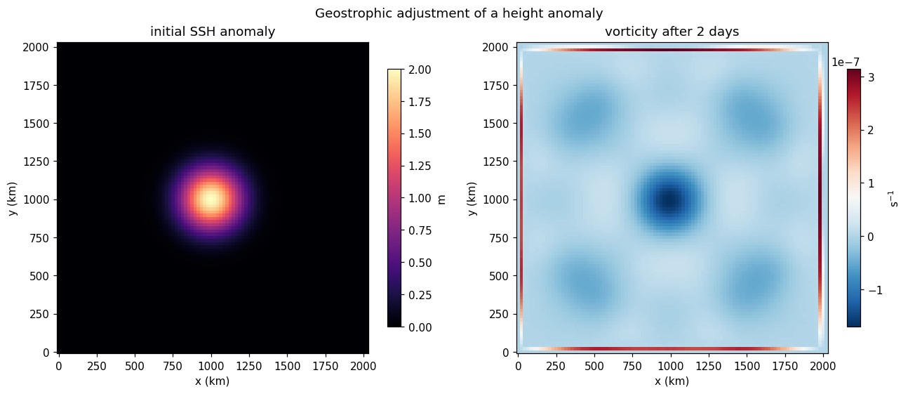
Geostrophic adjustment in the rotating shallow-water model –. Left: the initial sea-surface-height bump. Right: the relative vorticity after two days — a balanced rotating vortex has formed around the residual mound while gravity waves carry off the excess. — Figure 1:Geostrophic adjustment in the rotating shallow-water model (1)–(2). Left: the initial sea-surface-height bump. Right: the relative vorticity after two days — a balanced rotating vortex has formed around the residual mound while gravity waves carry off the excess.

3. Quasi-geostrophy and potential-vorticity dynamics¶

When the flow is slow compared to rotation (small Rossby number $\mathrm{Ro}=U/fL\ll 1$ ), the gravity waves filter out and the dynamics collapse onto a single prognostic scalar: the quasi-geostrophic potential vorticity (PV). For the barotropic model,

\partial_t q + J(\psi, q) = 0, \qquad q = \nabla^2\psi + \beta y,

(4)

where $\psi$ is the streamfunction, $J$ the advective Jacobian, and $\beta=\mathrm{d}f/\mathrm{d}y$ the planetary vorticity gradient. PV is materially conserved — advected, not created — and the velocity is recovered from $\psi$ by the same Poisson inversion $\nabla^2\psi=q-\beta y$ seen in Phase 2. somax discretises the Jacobian with the energy- and enstrophy-conserving Arakawa scheme Arakawa & Lamb (1977). We seed a vortex pair and let it self-advect.

qg = BarotropicQG.create(
    nx=96, ny=96, Lx=1e6, Ly=1e6, f0=1e-4, beta=1.6e-11, lateral_viscosity=50.0
)
xq = jnp.arange(qg.grid.Nx) * qg.grid.dx
yq = jnp.arange(qg.grid.Ny) * qg.grid.dy
Xq, Yq = jnp.meshgrid(xq, yq)
radius = 8e4
q0 = 1e-4 * (
    jnp.exp(-(((Xq - 6e5) ** 2 + (Yq - 5e5) ** 2) / radius**2))
    - jnp.exp(-(((Xq - 4e5) ** 2 + (Yq - 5e5) ** 2) / radius**2))
)
qg_state0 = qg.apply_boundary_conditions(BarotropicQGState(q=q0))

qg_sol = qg.integrate(qg_state0, t0=0.0, t1=5 * 86400.0, dt=900.0, max_steps=20000)
q_final = qg_sol.ys.q[-1]
qg_diag = qg.diagnose(BarotropicQGState(q=q_final))

Figure 2 shows the PV field after five days alongside the recovered streamfunction. The dipole has translated and sheared under mutual advection while conserving PV; the streamfunction contours are the instantaneous streamlines of the balanced flow.

fig, axes = plt.subplots(1, 2, figsize=(12, 5))
im0 = axes[0].pcolormesh(Xq / 1e3, Yq / 1e3, q_final, cmap="RdBu_r", shading="auto")
axes[0].set(
    xlabel="x (km)", ylabel="y (km)", title="potential vorticity $q$", aspect="equal"
)
fig.colorbar(im0, ax=axes[0], shrink=0.8)
im1 = axes[1].pcolormesh(
    Xq / 1e3, Yq / 1e3, qg_diag.psi, cmap="viridis", shading="auto"
)
axes[1].contour(
    Xq / 1e3, Yq / 1e3, qg_diag.psi, levels=12, colors="k", alpha=0.4, linewidths=0.6
)
axes[1].set(
    xlabel="x (km)", ylabel="y (km)", title=r"streamfunction $\psi$", aspect="equal"
)
fig.colorbar(im1, ax=axes[1], shrink=0.8)
fig.suptitle("Barotropic QG: a self-advecting vortex pair after 5 days")
fig.tight_layout()
fig.savefig(IMG_DIR / "qg_vortex.png", dpi=110, bbox_inches="tight")
plt.show()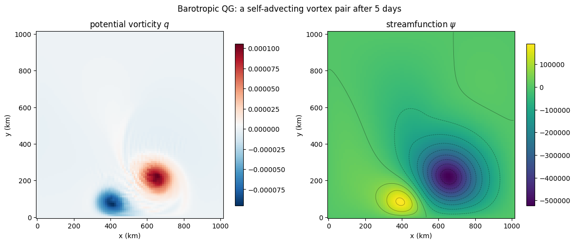

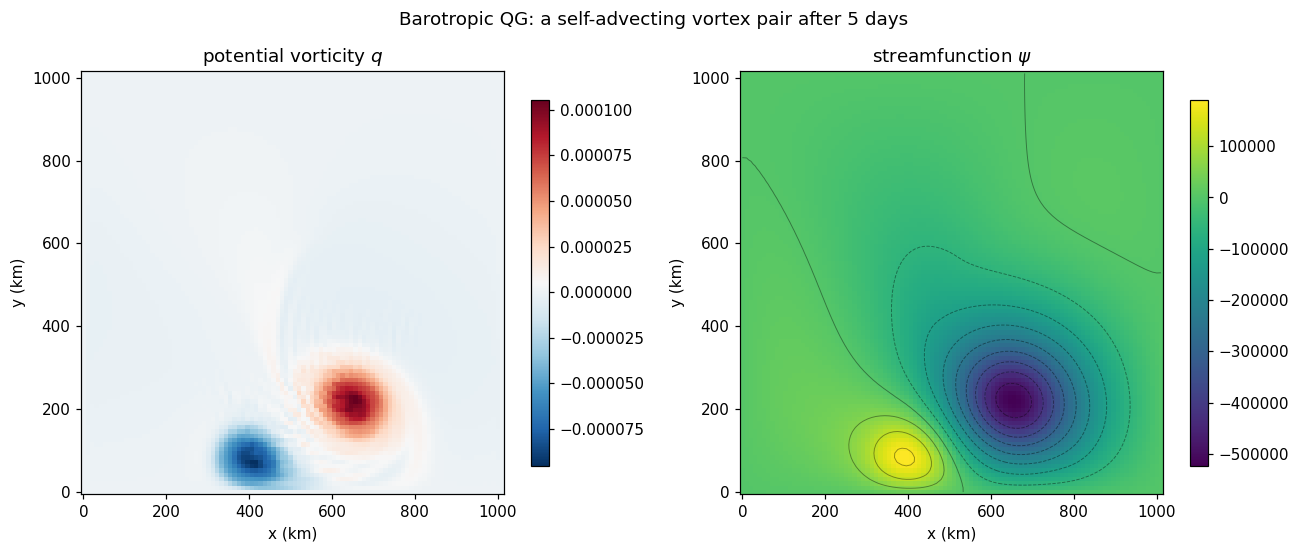
Barotropic quasi-geostrophic evolution of a vortex pair. Left: the materially-conserved PV after five days. Right: the streamfunction from the Poisson inversion, whose contours are the streamlines of the balanced flow. — Figure 2:Barotropic quasi-geostrophic evolution (4) of a vortex pair. Left: the materially-conserved PV after five days. Right: the streamfunction from the Poisson inversion, whose contours are the streamlines of the balanced flow.

Summary¶

The rotating shallow-water equations (1)–(2) add the Coriolis force; their fastest signal, the external gravity wave $c=\sqrt{gH}$ , sets the explicit CFL limit.
Geostrophic adjustment (3) is the defining rotating behaviour: a pressure anomaly settles into a balanced vortex of scale $L_d=\sqrt{gH}/f$ while radiating gravity waves.
The quasi-geostrophic reduction (4) filters the waves and reduces the dynamics to material advection of potential vorticity, recovered through the same elliptic inversion built in Phase 2 — the foundation of the multilayer ocean models and the data-assimilation studies that follow.

This completes the Phase 0–4 arc: from staggered grids and discrete operators, through the 1-D and 2-D building blocks and low-order chaos, to the rotating geophysical models that somax exists to solve. For running these models as configured simulations, see the somax-sim runner tutorial; for correcting them against observations, the data-assimilation tutorials.

References¶

Vallis, G. K. (2017). Atmospheric and oceanic fluid dynamics.
Cushman-Roisin, B., & Beckers, J.-M. (2011). Introduction to Geophysical Fluid Dynamics: Physical and Numerical Aspects (2nd ed., Vol. 101). Academic Press.
Pedlosky, J. (1987). Geophysical Fluid Dynamics (2nd ed.). Springer. 10.1007/978-1-4612-4650-3
Arakawa, A., & Lamb, V. R. (1977). Computational design of the basic dynamical processes of the UCLA general circulation model. Methods in Computational Physics, 17, 173–265.