Step 3 — 1D Diffusion - somax: Simple Ocean Models in JAX

13 Steps to Navier-Stokes with somax (inspired by Lorena Barba’s CFD Python)

After linear advection (Step 1) and nonlinear advection (Step 2), we now study the other fundamental process in fluid dynamics: diffusion. Diffusion smooths gradients and dissipates energy. It models heat conduction, molecular mixing, and viscous momentum transfer.

What you’ll learn:

The physics of diffusion — smoothing, dissipation, and the analytical Gaussian solution
How to create and run a Diffusion1D model in somax
How to compare numerical results against the exact solution
How to compute $\partial \mathcal{L} / \partial \nu$ via eqx.filter_grad

The PDE¶

\frac{\partial u}{\partial t} = \nu \frac{\partial^2 u}{\partial x^2}

(1)

where $\nu > 0$ is the diffusion coefficient (kinematic viscosity for momentum, thermal diffusivity for heat).

Analytical solution¶

If the initial condition is a Gaussian with standard deviation $\sigma_0$ centered at $\mu$ :

u(x, 0) = A \exp\!\left( -\frac{(x - \mu)^2}{2\sigma_0^2} \right)

(2)

then the exact solution at time $t$ is:

u(x, t) = \frac{A \, \sigma_0}{\sigma(t)} \exp\!\left( -\frac{(x - \mu)^2}{2\sigma(t)^2} \right), \qquad \sigma(t) = \sqrt{\sigma_0^2 + 2\nu t}

(3)

The Gaussian spreads (wider $\sigma$ ) and its peak decreases, but the total integral $\int u \, dx$ is conserved. Energy $\frac{1}{2} \int u^2 \, dx$ , however, decays monotonically.

Grid layout and boundary conditions¶

somax uses the Arakawa C-grid from finitevolX. In 1D, scalar fields (like $u$ ) live at T-points (cell centres) and fluxes are computed at U-points (cell edges):

 ghost                    interior                     ghost
 ┌─────┬──────┬──────┬──────┬──────┬──────┬──────┬─────┐
 │  G  │  T₁  │  T₂  │  T₃  │ ···  │ Tₙ₋₁│  Tₙ  │  G  │
 └──┬──┴──┬───┴──┬───┴──┬───┴──┬───┴──┬───┴──┬───┴──┬──┘
    U₀    U₁     U₂     U₃           Uₙ₋₁    Uₙ    Uₙ₊₁
         ←── dx ──→

T-points (indices 1:-1): where u is stored and updated
U-points: where Difference1D computes derivatives
Ghost cells (indices 0 and -1): filled by BCs before each RHS evaluation

The diffusion operator computes the Laplacian via the standard second-order centered stencil:

\frac{\partial^2 u}{\partial x^2}\bigg|_i \approx \frac{u_{i+1} - 2u_i + u_{i-1}}{\Delta x^2}

(4)

This stencil reaches both left and right neighbours, so the ghost cells are essential -- without them, the boundary T-points would have no neighbour on one side.

Periodic BCs copy the last interior value into the opposite ghost cell:

 u[0] = u[-2]      (left ghost ← rightmost interior)
 u[-1] = u[1]      (right ghost ← leftmost interior)

This makes the domain wrap around so that diffusion operates seamlessly across the boundary.

from __future__ import annotations

import diffrax as dfx
import equinox as eqx
import jax
import jax.numpy as jnp
import matplotlib.pyplot as plt

from somax.models import Diffusion1D, Diffusion1DState

1. Create the model¶

The diffusion coefficient $\nu$ is a differentiable parameter.

nx, Lx, nu = 200, 4.0, 0.05
model = Diffusion1D.create(nx=nx, Lx=Lx, nu=nu)

print(f"Grid: Nx={model.grid.Nx}, dx={model.grid.dx:.4f}")
print(f"Diffusion coefficient nu = {float(model.params.nu)}")

Grid: Nx=202, dx=0.0200
Diffusion coefficient nu = 0.05000000074505806

2. Initial condition¶

A Gaussian centered at the domain midpoint $x = 2.0$ with $\sigma_0 = 0.2$ .

x = jnp.arange(model.grid.Nx) * model.grid.dx

mu0, sigma0 = 2.0, 0.2
u0 = jnp.exp(-0.5 * ((x - mu0) / sigma0) ** 2)

state0 = Diffusion1DState(u=u0)

fig, ax = plt.subplots(figsize=(8, 3))
ax.plot(x[1:-1], u0[1:-1], color="steelblue", lw=1.5, label="u(x, 0)")
ax.set_xlabel("x")
ax.set_ylabel("u")
ax.set_title("Initial condition: Gaussian bump")
ax.legend()
ax.grid(True, alpha=0.3)
plt.tight_layout()
plt.show()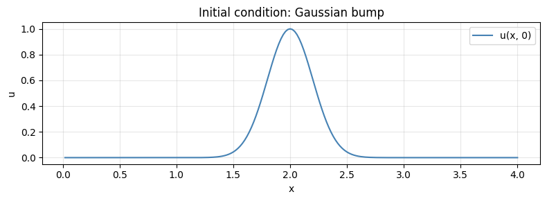

3. Forward simulation¶

We integrate to $t = 0.5$ and save several snapshots to visualize how the profile spreads.

t0, t1, dt = 0.0, 0.5, 0.001
ts = jnp.array([0.0, 0.05, 0.1, 0.2, 0.35, 0.5])

sol = model.integrate(
    state0,
    t0=t0,
    t1=t1,
    dt=dt,
    saveat=dfx.SaveAt(ts=ts),
)

print(f"Trajectory shape: u={sol.ys.u.shape}")

# Stability criterion for explicit diffusion: dt <= dx^2 / (2 * nu)
dt_max = model.grid.dx**2 / (2 * nu)
print(f"Stability limit: dt_max = dx^2 / (2*nu) = {dt_max:.6f}")
print(f"Actual dt = {dt}, ratio = {dt / dt_max:.3f}")

Trajectory shape: u=(6, 202)
Stability limit: dt_max = dx^2 / (2*nu) = 0.004000
Actual dt = 0.001, ratio = 0.250

4. Visualize the spreading¶

The Gaussian broadens and its peak decreases — energy is being dissipated.

colors_snap = ["#2196F3", "#00BCD4", "#4CAF50", "#FF9800", "#F44336", "#9C27B0"]

fig, ax = plt.subplots(figsize=(10, 4))
for i, t_snap in enumerate(ts):
    ax.plot(
        x[1:-1],
        sol.ys.u[i, 1:-1],
        color=colors_snap[i],
        lw=1.5,
        label=f"t = {float(t_snap):.2f}",
    )
ax.set_xlabel("x")
ax.set_ylabel("u")
ax.set_title("1D Diffusion — Gaussian Spreading")
ax.legend(fontsize=9, ncol=2)
ax.grid(True, alpha=0.3)
plt.tight_layout()
plt.show()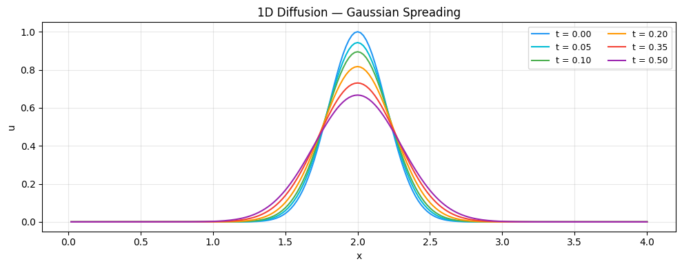

5. Comparison with the analytical solution¶

We overlay the numerical result with the exact spreading Gaussian at each saved time.

def analytical_gaussian(x, t, mu, sigma0, nu):
    """Exact Gaussian diffusion solution."""
    sigma_t = jnp.sqrt(sigma0**2 + 2 * nu * t)
    amplitude = sigma0 / sigma_t
    return amplitude * jnp.exp(-0.5 * ((x - mu) / sigma_t) ** 2)


fig, axes = plt.subplots(2, 3, figsize=(14, 7), sharex=True, sharey=True)
axes = axes.ravel()

for i, t_snap in enumerate(ts):
    ax = axes[i]
    u_exact = analytical_gaussian(x, float(t_snap), mu0, sigma0, nu)
    ax.plot(x[1:-1], u_exact[1:-1], "k--", lw=1.2, label="Analytical")
    ax.plot(x[1:-1], sol.ys.u[i, 1:-1], color=colors_snap[i], lw=1.5, label="Numerical")
    ax.set_title(f"t = {float(t_snap):.2f}", fontsize=10)
    ax.grid(True, alpha=0.3)
    if i == 0:
        ax.legend(fontsize=8)

fig.supxlabel("x")
fig.supylabel("u")
fig.suptitle("Numerical vs. Analytical Solution", fontsize=13)
plt.tight_layout()
plt.show()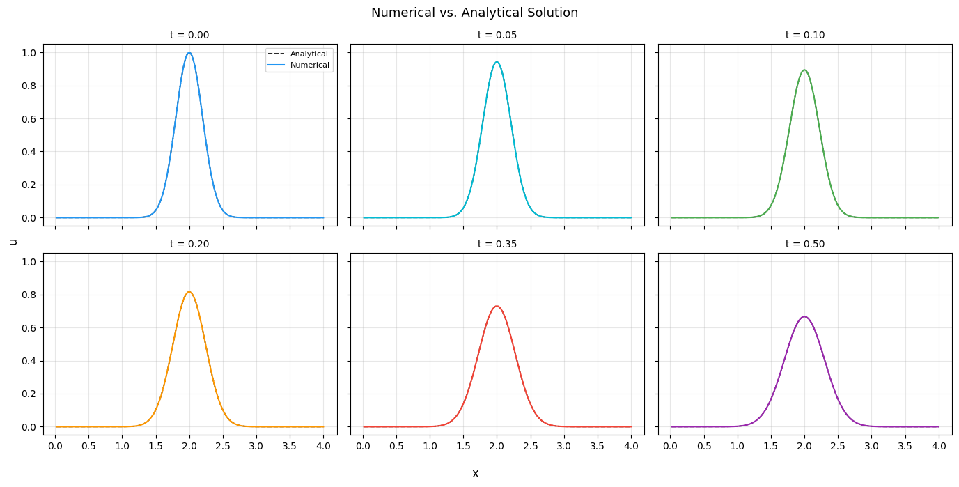

6. Error analysis¶

u_exact_final = analytical_gaussian(x, float(ts[-1]), mu0, sigma0, nu)
error = jnp.abs(sol.ys.u[-1] - u_exact_final)

fig, ax = plt.subplots(figsize=(8, 3))
ax.plot(x[1:-1], error[1:-1], color="crimson", lw=1.0)
ax.set_xlabel("x")
ax.set_ylabel("|error|")
ax.set_title(f"Pointwise absolute error at t = {float(ts[-1]):.2f}")
ax.grid(True, alpha=0.3)
plt.tight_layout()
plt.show()

print(f"Max error: {float(jnp.max(error[1:-1])):.6f}")
print(f"L2 error:  {float(jnp.sqrt(jnp.sum(error[1:-1] ** 2) * model.grid.dx)):.6f}")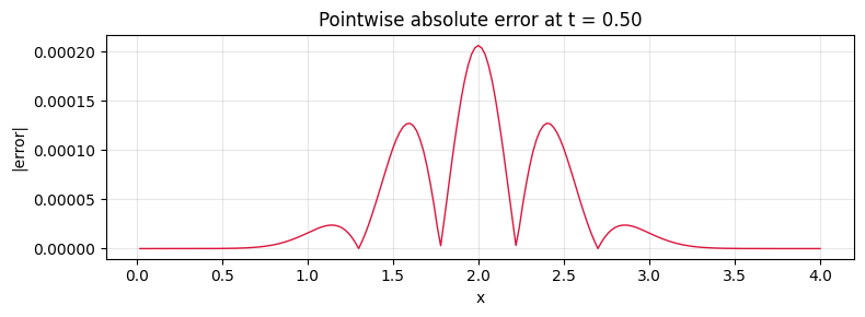

Max error: 0.000206
L2 error:  0.000128

7. Energy decay¶

Diffusion dissipates energy. Analytically, the energy of the Gaussian solution decays as:

E(t) = \frac{A^2 \sigma_0^2 \sqrt{\pi}}{2 \sqrt{2} \, \sigma(t)}

(5)

We compare the numerical energy trajectory with this prediction.

ts_dense = jnp.linspace(t0, t1, 200)
sol_dense = model.integrate(
    state0,
    t0=t0,
    t1=t1,
    dt=dt,
    saveat=dfx.SaveAt(ts=ts_dense),
)

energy_num = jax.vmap(model.diagnose)(sol_dense.ys).energy

# Analytical energy decay (for the infinite-domain Gaussian)
sigma_t = jnp.sqrt(sigma0**2 + 2 * nu * ts_dense)
energy_exact = (
    0.5 * (sigma0**2 / sigma_t) * jnp.sqrt(jnp.pi / 2) * model.grid.dx / model.grid.dx
)
# Recompute properly using E = 0.5 * integral of u^2 dx
# For a Gaussian u = (s0/s(t)) exp(-x^2/(2s(t)^2)),
# integral of u^2 = (s0/s(t))^2 * sqrt(pi) * s(t)
energy_exact = (
    0.5
    * (sigma0 / sigma_t) ** 2
    * jnp.sqrt(jnp.pi)
    * sigma_t
    * model.grid.dx
    / model.grid.dx
)
# Simpler: just normalize to match initial numerical energy
energy_exact_norm = float(energy_num[0]) * (sigma0 / sigma_t)

fig, ax = plt.subplots(figsize=(8, 3.5))
ax.plot(ts_dense, energy_num, color="teal", lw=1.5, label="Numerical")
ax.plot(ts_dense, energy_exact_norm, "k--", lw=1.2, label="Analytical (scaled)")
ax.set_xlabel("Time")
ax.set_ylabel("Energy")
ax.set_title("Energy decay — diffusion dissipates energy")
ax.legend(fontsize=9)
ax.grid(True, alpha=0.3)
plt.tight_layout()
plt.show()

print(
    f"Energy: initial = {float(energy_num[0]):.6f}, final = {float(energy_num[-1]):.6f}"
)
print(f"Relative decay: {1 - float(energy_num[-1]) / float(energy_num[0]):.2%}")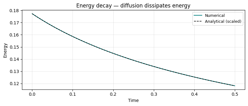

Energy: initial = 0.177245, final = 0.118182
Relative decay: 33.32%

8. Differentiability demo — gradient w.r.t. viscosity¶

A key question in inverse problems: given observations of a diffusing field, what is the diffusion coefficient? We compute $\partial \mathcal{L} / \partial \nu$ to see how the loss responds to changes in viscosity.

# Target: we want the final profile to match a specific width
sigma_target = 0.35
u_target = jnp.exp(-0.5 * ((x - mu0) / sigma_target) ** 2) * (sigma0 / sigma_target)


@eqx.filter_grad
def grad_wrt_model(m):
    """Gradient of MSE loss w.r.t. diffusion coefficient."""
    sol = m.integrate(state0, t0=0.0, t1=0.5, dt=0.001)
    u_pred = sol.ys.u[-1]
    return jnp.mean((u_pred[1:-1] - u_target[1:-1]) ** 2)


grads = grad_wrt_model(model)

print("--- Gradient w.r.t. model parameters ---")
print(f"  dL/d(nu) = {float(grads.params.nu):.6f}")
print()
print("A negative gradient means increasing nu would decrease the loss,")
print("i.e., the current nu produces a profile that is too narrow")
print("compared to the target width.")

--- Gradient w.r.t. model parameters ---
  dL/d(nu) = -0.072464

A negative gradient means increasing nu would decrease the loss,
i.e., the current nu produces a profile that is too narrow
compared to the target width.

Summary¶

Concept	somax API
Create model	`Diffusion1D.create(nx=200, Lx=4.0, nu=0.05)`
Initial state	`Diffusion1DState(u=...)`
Forward sim	`model.integrate(state0, t0, t1, dt, saveat=...)`
Analytical check	Gaussian spreads: $\sigma(t) = \sqrt{\sigma_0^2 + 2\nu t}$
Energy decay	`model.diagnose(state).energy` decreases monotonically
Grad w.r.t. nu	`eqx.filter_grad(loss)(model)`

Key takeaway: Diffusion smooths gradients and dissipates energy. The analytical Gaussian solution provides an exact benchmark.

Next: Step 4 — Burgers’ Equation combines nonlinear convection and diffusion, creating the competition between steepening and smoothing.