Step 6 -- 2D Nonlinear Convection - somax: Simple Ocean Models in JAX

We now replace the constant advection velocity with the solution itself, giving the 2D nonlinear convection (inviscid Burgers) system:

\frac{\partial u}{\partial t} + u \frac{\partial u}{\partial x} + v \frac{\partial u}{\partial y} = 0

(1)

\frac{\partial v}{\partial t} + u \frac{\partial v}{\partial x} + v \frac{\partial v}{\partial y} = 0

(2)

What you will learn:

How nonlinear self-advection produces wave steepening in 2D
Working with two-component state vectors $(u, v)$
How the solution differs from the linear case

Physics¶

In the linear case (Step 5) the wave translates at constant speed without changing shape. Here the local propagation speed is the solution: regions of higher amplitude travel faster, causing the wave front to steepen. Without viscosity, this eventually leads to a shock (gradient blow-up). In practice we run for a short time to observe the steepening before any numerical instability.

Grid layout and boundary conditions¶

In 2D, somax uses the Arakawa C-grid where different variables live at different positions within each cell:

       V_{j+1/2}
    ┌─────●─────┐
    │           │
 U  ●     T     ●  U
i-1/2   (i,j)    i+1/2
    │           │
    └─────●─────┘
       V_{j-1/2}

T-points (cell centres): scalars ( $u$ , $p$ , $\omega$ )
U-points (east/west faces): x-fluxes
V-points (north/south faces): y-fluxes
X-points (corners): vorticity (in some formulations)

The full array has shape (Ny, Nx) with a 1-cell ghost ring on all sides:

 ┌───────────────────────────────────┐
 │  ghost  ghost  ghost  ghost  ghost│  ← row 0
 │  ghost  T(1,1) T(1,2) ···   ghost│  ← row 1
 │  ghost  T(2,1) T(2,2) ···   ghost│
 │   ⋮      ⋮      ⋮           ⋮    │
 │  ghost  T(n,1) T(n,2) ···   ghost│  ← row Ny-2
 │  ghost  ghost  ghost  ghost  ghost│  ← row Ny-1
 └───────────────────────────────────┘
        col 0  col 1  ···  col Nx-1

Interior cells are [1:-1, 1:-1]. Ghost cells are filled by boundary conditions before each RHS evaluation.

Periodic BCs (enforce_periodic) copy the last interior row/column to the opposite ghost row/column. Both u and v fields receive the same periodic treatment:

 field[0, :]  = field[-2, :]   (south ghost ← north interior)
 field[-1, :] = field[1, :]    (north ghost ← south interior)
 field[:, 0]  = field[:, -2]   (west ghost ← east interior)
 field[:, -1] = field[:, 1]    (east ghost ← west interior)

from __future__ import annotations

import diffrax as dfx
import jax
import jax.numpy as jnp
import matplotlib.pyplot as plt

from somax.models import NonlinearConvection2D, NonlinearConvection2DState

1. Create the model¶

model = NonlinearConvection2D.create(nx=64, ny=64)
print(model)
print(f"Grid: Nx={model.grid.Nx}, Ny={model.grid.Ny}")
print(f"Spacing: dx={model.grid.dx:.4f}, dy={model.grid.dy:.4f}")

NonlinearConvection2D(
  grid=ArakawaCGrid2D(Nx=66, Ny=66, Lx=2.0, Ly=2.0, dx=0.03125, dy=0.03125),
  advection=Advection2D(
    grid=ArakawaCGrid2D(Nx=66, Ny=66, Lx=2.0, Ly=2.0, dx=0.03125, dy=0.03125),
    recon=Reconstruction2D(
      grid=ArakawaCGrid2D(Nx=66, Ny=66, Lx=2.0, Ly=2.0, dx=0.03125, dy=0.03125)
    )
  ),
  interp=Interpolation2D(
    grid=ArakawaCGrid2D(Nx=66, Ny=66, Lx=2.0, Ly=2.0, dx=0.03125, dy=0.03125)
  )
)
Grid: Nx=66, Ny=66
Spacing: dx=0.0312, dy=0.0312

2. Initial condition¶

A 2D Gaussian for both velocity components, centred at $(1.0, 1.0)$ .

x = jnp.arange(model.grid.Nx) * model.grid.dx
y = jnp.arange(model.grid.Ny) * model.grid.dy
X, Y = jnp.meshgrid(x, y)

sigma0 = 0.2
gauss = jnp.exp(-0.5 * (((X - 1.0) / sigma0) ** 2 + ((Y - 1.0) / sigma0) ** 2))
u0 = gauss
v0 = gauss

state0 = NonlinearConvection2DState(u=u0, v=v0)
print(f"State shapes: u={state0.u.shape}, v={state0.v.shape}")

State shapes: u=(66, 66), v=(66, 66)

3. Run the simulation¶

dt = 0.002
t_final = 0.3
ts = jnp.arange(0.0, t_final, dt)

sol = model.integrate(
    state0,
    t0=0.0,
    t1=t_final,
    dt=dt,
    saveat=dfx.SaveAt(ts=ts),
)

print(f"Solution shapes: u={sol.ys.u.shape}, v={sol.ys.v.shape}")

Solution shapes: u=(150, 66, 66), v=(150, 66, 66)

4. Visualize steepening¶

Compare the initial and final $u$ and $v$ fields. The Gaussian should steepen on one side as faster-moving peaks overtake slower regions.

fig, axes = plt.subplots(2, 2, figsize=(12, 10))

fields = [
    (sol.ys.u[0], "u -- initial"),
    (sol.ys.u[-1], f"u -- t = {float(ts[-1]):.2f}"),
    (sol.ys.v[0], "v -- initial"),
    (sol.ys.v[-1], f"v -- t = {float(ts[-1]):.2f}"),
]

for ax, (field, title) in zip(axes.ravel(), fields, strict=True):
    pcm = ax.pcolormesh(
        X[1:-1, 1:-1],
        Y[1:-1, 1:-1],
        field[1:-1, 1:-1],
        shading="auto",
        cmap="viridis",
    )
    plt.colorbar(pcm, ax=ax)
    ax.set_xlabel("x")
    ax.set_ylabel("y")
    ax.set_title(title)
    ax.set_aspect("equal")

plt.suptitle("2D Nonlinear Convection -- Wave Steepening", fontsize=14)
plt.tight_layout()
plt.show()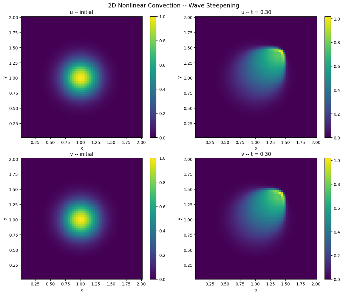

5. Cross-sections through the steepening front¶

Taking a 1D slice through the middle row makes the steepening easier to see.

mid_y = model.grid.Ny // 2

fig, axes = plt.subplots(1, 2, figsize=(12, 4))

# u cross-section
axes[0].plot(x[1:-1], sol.ys.u[0, mid_y, 1:-1], label="t = 0", lw=1.5)
axes[0].plot(
    x[1:-1],
    sol.ys.u[-1, mid_y, 1:-1],
    label=f"t = {float(ts[-1]):.2f}",
    lw=1.5,
    ls="--",
)
axes[0].set_xlabel("x")
axes[0].set_ylabel("u")
axes[0].set_title("u cross-section at mid-y")
axes[0].legend()
axes[0].grid(True, alpha=0.3)

# v cross-section
mid_x = model.grid.Nx // 2
axes[1].plot(y[1:-1], sol.ys.v[0, 1:-1, mid_x], label="t = 0", lw=1.5)
axes[1].plot(
    y[1:-1],
    sol.ys.v[-1, 1:-1, mid_x],
    label=f"t = {float(ts[-1]):.2f}",
    lw=1.5,
    ls="--",
)
axes[1].set_xlabel("y")
axes[1].set_ylabel("v")
axes[1].set_title("v cross-section at mid-x")
axes[1].legend()
axes[1].grid(True, alpha=0.3)

plt.tight_layout()
plt.show()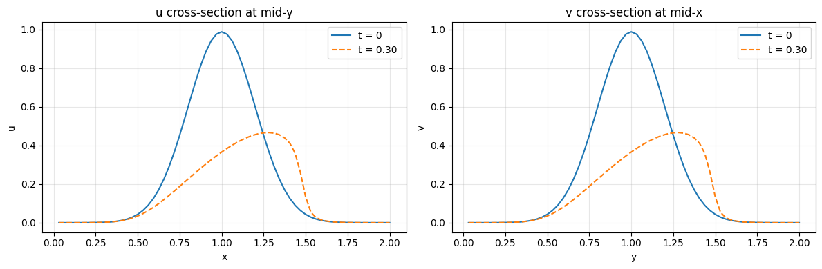

6. Compare with linear convection¶

In the linear case (Step 5) the peak amplitude is preserved. Here self-advection redistributes energy and the peak drops as the front steepens.

peak_u = jnp.max(sol.ys.u[:, 1:-1, 1:-1], axis=(1, 2))

fig, ax = plt.subplots(figsize=(8, 4))
ax.plot(ts, peak_u, lw=1.5, color="#F44336")
ax.set_xlabel("Time")
ax.set_ylabel("max(u)")
ax.set_title("Peak amplitude decay from nonlinear steepening")
ax.grid(True, alpha=0.3)
plt.tight_layout()
plt.show()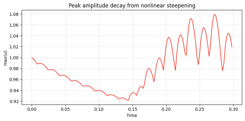

7. Energy evolution¶

Total kinetic energy $E = \tfrac{1}{2}\sum(u^2 + v^2)\,dx\,dy$ should not increase for this inviscid system (numerical dissipation may cause a slight decrease).

dx_val, dy_val = float(model.grid.dx), float(model.grid.dy)
energy = (
    0.5
    * jnp.sum(
        sol.ys.u[:, 1:-1, 1:-1] ** 2 + sol.ys.v[:, 1:-1, 1:-1] ** 2,
        axis=(1, 2),
    )
    * dx_val
    * dy_val
)

fig, ax = plt.subplots(figsize=(8, 3))
ax.plot(ts, energy, lw=1.5, color="#9C27B0")
ax.set_xlabel("Time")
ax.set_ylabel("Kinetic energy")
ax.set_title("Energy evolution (inviscid -- should be roughly constant)")
ax.grid(True, alpha=0.3)
plt.tight_layout()
plt.show()

print(f"Energy: initial = {float(energy[0]):.6f}, final = {float(energy[-1]):.6f}")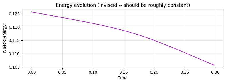

Energy: initial = 0.125664, final = 0.105718

8. Gradient through the initial state¶

Even without explicit parameters, we can differentiate through the nonlinear dynamics with respect to the initial condition.

def loss_state(s0):
    sol = model.integrate(s0, t0=0.0, t1=0.1, dt=0.002)
    return jnp.sum(sol.ys.u**2 + sol.ys.v**2)


grad_s0 = jax.grad(loss_state)(state0)

fig, axes = plt.subplots(1, 2, figsize=(12, 5))

pcm0 = axes[0].pcolormesh(
    X[1:-1, 1:-1],
    Y[1:-1, 1:-1],
    grad_s0.u[1:-1, 1:-1],
    shading="auto",
    cmap="RdBu_r",
)
plt.colorbar(pcm0, ax=axes[0])
axes[0].set_title("dL/du0")
axes[0].set_xlabel("x")
axes[0].set_ylabel("y")
axes[0].set_aspect("equal")

pcm1 = axes[1].pcolormesh(
    X[1:-1, 1:-1],
    Y[1:-1, 1:-1],
    grad_s0.v[1:-1, 1:-1],
    shading="auto",
    cmap="RdBu_r",
)
plt.colorbar(pcm1, ax=axes[1])
axes[1].set_title("dL/dv0")
axes[1].set_xlabel("x")
axes[1].set_ylabel("y")
axes[1].set_aspect("equal")

plt.suptitle("Adjoint sensitivity of nonlinear convection", fontsize=14)
plt.tight_layout()
plt.show()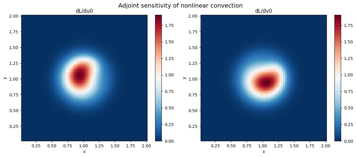

Summary¶

Concept	API
Create model	`NonlinearConvection2D.create(nx=64, ny=64)`
Two-component state	`NonlinearConvection2DState(u=u0, v=v0)`
Self-advection	velocity = solution itself
Observable effect	wave steepening, peak decay

Next: Step 7 adds diffusion in 2D, which counteracts steepening and has an analytical Gaussian solution we can validate against.