Step 8 -- 2D Burgers’ Equation - somax: Simple Ocean Models in JAX

The 2D viscous Burgers equation combines nonlinear convection (Step 6) with diffusion (Step 7):

\frac{\partial u}{\partial t} + u \frac{\partial u}{\partial x} + v \frac{\partial u}{\partial y} = \nu \left( \frac{\partial^2 u}{\partial x^2} + \frac{\partial^2 u}{\partial y^2} \right)

(1)

\frac{\partial v}{\partial t} + u \frac{\partial v}{\partial x} + v \frac{\partial v}{\partial y} = \nu \left( \frac{\partial^2 v}{\partial x^2} + \frac{\partial^2 v}{\partial y^2} \right)

(2)

What you will learn:

How viscosity balances nonlinear steepening
The effect of low vs. high viscosity on the solution
Differentiating through $\nu$ for parameter sensitivity
Why Burgers is the gateway to Navier--Stokes

Physics¶

Burgers’ equation is the simplest PDE that contains both nonlinear advection and diffusion -- the same two ingredients that appear in the Navier--Stokes momentum equation. Low viscosity allows steep gradients (near-shocks); high viscosity smooths everything out. The balance between these two effects determines the solution character and is controlled by the Reynolds number $\mathrm{Re} = U L / \nu$ .

Grid layout and boundary conditions¶

In 2D, somax uses the Arakawa C-grid where different variables live at different positions within each cell:

       V_{j+1/2}
    ┌─────●─────┐
    │           │
 U  ●     T     ●  U
i-1/2   (i,j)    i+1/2
    │           │
    └─────●─────┘
       V_{j-1/2}

T-points (cell centres): scalars ( $u$ , $p$ , $\omega$ )
U-points (east/west faces): x-fluxes
V-points (north/south faces): y-fluxes
X-points (corners): vorticity (in some formulations)

The full array has shape (Ny, Nx) with a 1-cell ghost ring on all sides:

 ┌───────────────────────────────────┐
 │  ghost  ghost  ghost  ghost  ghost│  ← row 0
 │  ghost  T(1,1) T(1,2) ···   ghost│  ← row 1
 │  ghost  T(2,1) T(2,2) ···   ghost│
 │   ⋮      ⋮      ⋮           ⋮    │
 │  ghost  T(n,1) T(n,2) ···   ghost│  ← row Ny-2
 │  ghost  ghost  ghost  ghost  ghost│  ← row Ny-1
 └───────────────────────────────────┘
        col 0  col 1  ···  col Nx-1

Interior cells are [1:-1, 1:-1]. Ghost cells are filled by boundary conditions before each RHS evaluation.

Periodic BCs (enforce_periodic) copy the last interior row/column to the opposite ghost row/column. Both u and v fields receive the same periodic treatment:

 field[0, :]  = field[-2, :]   (south ghost ← north interior)
 field[-1, :] = field[1, :]    (north ghost ← south interior)
 field[:, 0]  = field[:, -2]   (west ghost ← east interior)
 field[:, -1] = field[:, 1]    (east ghost ← west interior)

from __future__ import annotations

import diffrax as dfx
import equinox as eqx
import jax
import jax.numpy as jnp
import matplotlib.pyplot as plt

from somax.models import Burgers2D, Burgers2DState

1. Create the model¶

model = Burgers2D.create(nx=64, ny=64, Lx=2.0, Ly=2.0, nu=0.05)
print(model)
print(f"Grid: Nx={model.grid.Nx}, Ny={model.grid.Ny}")
print(f"Spacing: dx={model.grid.dx:.4f}, dy={model.grid.dy:.4f}")

Burgers2D(
  params=Burgers2DParams(nu=weak_f32[]),
  grid=ArakawaCGrid2D(Nx=66, Ny=66, Lx=2.0, Ly=2.0, dx=0.03125, dy=0.03125),
  diff=Difference2D(
    grid=ArakawaCGrid2D(Nx=66, Ny=66, Lx=2.0, Ly=2.0, dx=0.03125, dy=0.03125)
  ),
  advection=Advection2D(
    grid=ArakawaCGrid2D(Nx=66, Ny=66, Lx=2.0, Ly=2.0, dx=0.03125, dy=0.03125),
    recon=Reconstruction2D(
      grid=ArakawaCGrid2D(Nx=66, Ny=66, Lx=2.0, Ly=2.0, dx=0.03125, dy=0.03125)
    )
  ),
  interp=Interpolation2D(
    grid=ArakawaCGrid2D(Nx=66, Ny=66, Lx=2.0, Ly=2.0, dx=0.03125, dy=0.03125)
  )
)
Grid: Nx=66, Ny=66
Spacing: dx=0.0312, dy=0.0312

2. Initial condition¶

A 2D Gaussian for both velocity components.

x = jnp.arange(model.grid.Nx) * model.grid.dx
y = jnp.arange(model.grid.Ny) * model.grid.dy
X, Y = jnp.meshgrid(x, y)

sigma0 = 0.2
gauss = jnp.exp(-0.5 * (((X - 1.0) / sigma0) ** 2 + ((Y - 1.0) / sigma0) ** 2))
u0 = gauss
v0 = gauss

state0 = Burgers2DState(u=u0, v=v0)
print(f"State shapes: u={state0.u.shape}, v={state0.v.shape}")

State shapes: u=(66, 66), v=(66, 66)

3. Run the simulation¶

dt = 0.002
t_final = 0.5
ts = jnp.arange(0.0, t_final, dt)

sol = model.integrate(
    state0,
    t0=0.0,
    t1=t_final,
    dt=dt,
    saveat=dfx.SaveAt(ts=ts),
)

print(f"Solution shapes: u={sol.ys.u.shape}, v={sol.ys.v.shape}")

Solution shapes: u=(250, 66, 66), v=(250, 66, 66)

4. Visualize initial and final fields¶

fig, axes = plt.subplots(1, 3, figsize=(16, 4.5))

pcm0 = axes[0].pcolormesh(
    X[1:-1, 1:-1],
    Y[1:-1, 1:-1],
    sol.ys.u[0, 1:-1, 1:-1],
    shading="auto",
    cmap="viridis",
)
plt.colorbar(pcm0, ax=axes[0])
axes[0].set_title("u -- initial")
axes[0].set_xlabel("x")
axes[0].set_ylabel("y")
axes[0].set_aspect("equal")

pcm1 = axes[1].pcolormesh(
    X[1:-1, 1:-1],
    Y[1:-1, 1:-1],
    sol.ys.u[-1, 1:-1, 1:-1],
    shading="auto",
    cmap="viridis",
)
plt.colorbar(pcm1, ax=axes[1])
axes[1].set_title(f"u -- t = {float(ts[-1]):.2f}")
axes[1].set_xlabel("x")
axes[1].set_ylabel("y")
axes[1].set_aspect("equal")

pcm2 = axes[2].pcolormesh(
    X[1:-1, 1:-1],
    Y[1:-1, 1:-1],
    sol.ys.v[-1, 1:-1, 1:-1],
    shading="auto",
    cmap="viridis",
)
plt.colorbar(pcm2, ax=axes[2])
axes[2].set_title(f"v -- t = {float(ts[-1]):.2f}")
axes[2].set_xlabel("x")
axes[2].set_ylabel("y")
axes[2].set_aspect("equal")

plt.suptitle(r"2D Burgers ($\nu$ = 0.05)", fontsize=14)
plt.tight_layout()
plt.show()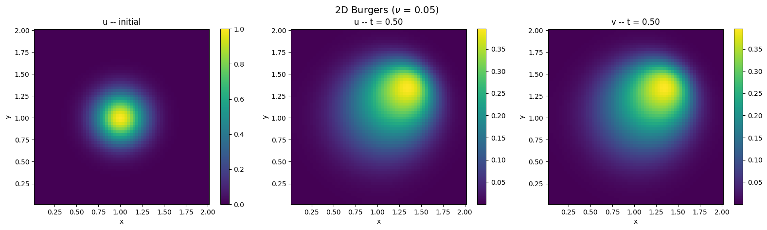

5. Low vs. high viscosity¶

We run two simulations with different viscosities from the same initial condition and compare the final fields.

nu_low, nu_high = 0.01, 0.2

model_low = Burgers2D.create(nx=64, ny=64, Lx=2.0, Ly=2.0, nu=nu_low)
model_high = Burgers2D.create(nx=64, ny=64, Lx=2.0, Ly=2.0, nu=nu_high)

sol_low = model_low.integrate(
    state0,
    t0=0.0,
    t1=t_final,
    dt=dt,
    saveat=dfx.SaveAt(t1=True),
)
sol_high = model_high.integrate(
    state0,
    t0=0.0,
    t1=t_final,
    dt=dt,
    saveat=dfx.SaveAt(t1=True),
)

fig, axes = plt.subplots(1, 2, figsize=(12, 5))

pcm0 = axes[0].pcolormesh(
    X[1:-1, 1:-1],
    Y[1:-1, 1:-1],
    sol_low.ys.u[0, 1:-1, 1:-1],
    shading="auto",
    cmap="viridis",
)
plt.colorbar(pcm0, ax=axes[0])
axes[0].set_title(rf"Low viscosity ($\nu$ = {nu_low})")
axes[0].set_xlabel("x")
axes[0].set_ylabel("y")
axes[0].set_aspect("equal")

pcm1 = axes[1].pcolormesh(
    X[1:-1, 1:-1],
    Y[1:-1, 1:-1],
    sol_high.ys.u[0, 1:-1, 1:-1],
    shading="auto",
    cmap="viridis",
)
plt.colorbar(pcm1, ax=axes[1])
axes[1].set_title(rf"High viscosity ($\nu$ = {nu_high})")
axes[1].set_xlabel("x")
axes[1].set_ylabel("y")
axes[1].set_aspect("equal")

plt.suptitle(f"Burgers 2D at t = {t_final} -- viscosity comparison", fontsize=14)
plt.tight_layout()
plt.show()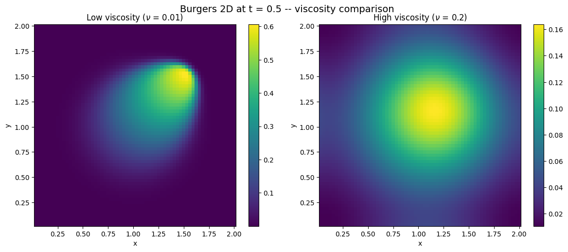

Low viscosity preserves sharper gradients (the nonlinear steepening from Step 6 dominates). High viscosity smears the solution out (the diffusion from Step 7 dominates).

6. Cross-section comparison¶

mid_y = model.grid.Ny // 2

fig, ax = plt.subplots(figsize=(8, 4))
ax.plot(x[1:-1], u0[mid_y, 1:-1], label="Initial", lw=1.5, color="black", ls=":")
ax.plot(
    x[1:-1],
    sol_low.ys.u[0, mid_y, 1:-1],
    label=rf"$\nu$ = {nu_low}",
    lw=1.5,
    color="#E53935",
)
ax.plot(
    x[1:-1],
    sol_high.ys.u[0, mid_y, 1:-1],
    label=rf"$\nu$ = {nu_high}",
    lw=1.5,
    color="#1E88E5",
)
ax.set_xlabel("x")
ax.set_ylabel("u")
ax.set_title(f"u cross-section at mid-y, t = {t_final}")
ax.legend()
ax.grid(True, alpha=0.3)
plt.tight_layout()
plt.show()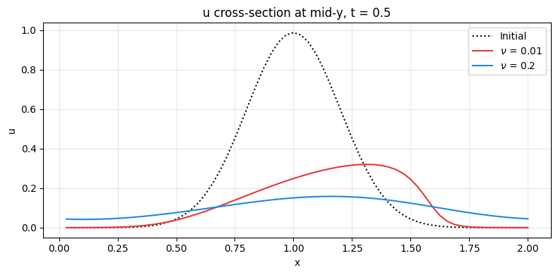

7. Gradient through viscosity¶

We compute $\partial \mathcal{L} / \partial \nu$ where $\mathcal{L} = \sum (u^2 + v^2)$ . This tells us how the total kinetic energy depends on viscosity -- useful for calibrating sub-grid diffusion.

@eqx.filter_grad
def grad_nu(m):
    sol = m.integrate(state0, t0=0.0, t1=0.3, dt=0.002)
    return jnp.sum(sol.ys.u**2 + sol.ys.v**2)


grads = grad_nu(model)

print("--- Gradient w.r.t. viscosity ---")
print(f"  dL/d(nu) = {grads.params.nu:.6f}")

--- Gradient w.r.t. viscosity ---

  dL/d(nu) = -1006.128723

8. Joint gradient -- viscosity and initial state¶

def loss_joint(s0, m):
    sol = m.integrate(s0, t0=0.0, t1=0.3, dt=0.002)
    return jnp.sum(sol.ys.u**2 + sol.ys.v**2)


grads_s0, grads_m = jax.grad(loss_joint, argnums=(0, 1))(state0, model)

print("--- Joint gradient ---")
print(f"  max |dL/du0| = {float(jnp.max(jnp.abs(grads_s0.u))):.6f}")
print(f"  max |dL/dv0| = {float(jnp.max(jnp.abs(grads_s0.v))):.6f}")
print(f"  dL/d(nu)     = {grads_m.params.nu:.6f}")

--- Joint gradient ---
  max |dL/du0| = 0.735805
  max |dL/dv0| = 0.735805
  dL/d(nu)     = -1006.128723

Summary¶

Concept	API
Create model	`Burgers2D.create(nx=64, ny=64, Lx=2.0, Ly=2.0, nu=0.05)`
Two-component state	`Burgers2DState(u=u0, v=v0)`
Viscosity comparison	create two models with different `nu`
Grad w.r.t. $\nu$	`eqx.filter_grad(loss)(model)`
Joint grad	`jax.grad(loss, argnums=(0, 1))(state0, model)`

Where we stand: Steps 5--8 have covered the fundamental building blocks of fluid dynamics in 2D: linear advection, nonlinear advection, diffusion, and their combination in Burgers’ equation. The next steps introduce elliptic solvers (Laplace, Poisson) which are needed to enforce incompressibility in the Navier--Stokes equations.