The six-step cycle
Report 17 · The data-driven modeling cycle is the benchmark ladder, run on one retrieval
Abstract¶
The scoping report organises the road from a forward model to an amortized predictor as the six-step cycle (overview). It makes step 2 (the classical inversion) the permanent oracle that validates steps 3 to 5, and it proposes a CycleStageBenchmark, a model-role enum and a lineage record. In this page, we run all six steps on the pinned code for one row of the cycle matrix, the L1 → L2 retrieval of a methane column from five-band transmittances. The cycle is already there, as pipekit-evaluate ships it as its benchmark ladder, with six rungs and a reference rule which scores the emulator against the simulator and both fast inversions against the oracle. The run shows why that rule matters. An emulator within 3.2 % of the simulator moves the posterior by up to 1.9 standard deviations and barely changes its coverage of the truth, whereas an amortized predictor that passes against the truth is 53 % too wide against the oracle where the column is small. What is missing is small, which is 1) a cell that names a transition, 2) an oracle strength, 3) a way to score the emulator on its inputs (what the ladder calls parameters), and 4) lineage that the registry cannot overwrite. Every number below is from a real run.
About this report
| Status | Mostly built. Originally a scoping proposal (“committed”: the cycle as a third organising axis, step 2 as oracle, a CycleStageBenchmark in pipekit-evaluate v0.2); the cycle and the oracle are kept, the new classes are replaced by the shipped ladder and three small extensions |
| Reading time | about 25 minutes |
| Audience | anyone taking a method from “we have a forward model” to “we have a deployed predictor”, and anyone deciding what a step must reproduce before the next one is trusted |
| Companions | Report 14 (pipekit-evaluate and the ladder); Report 15 (the benchmark contract); Report 11 (emulators and amortized retrievals on the same sensor); Report 10 (the Gauss–Newton retrieval); Report 12 (the registry); the overview and the benchmarks gallery |
| Code checked against | pipekit 0.0.2 at ef3c17f (pipekit, pipekit-cycle, pipekit-train, pipekit-experiment, pipekit-evaluate and its benchmark_ladder.md); xrtoolz 0.0.5 at 308c7f2; geotoolz 0.10.2 at 088475e. Read on 14 October 2026 |
| Running example | every output is from one run of notebooks/reports/report17_cycle.py, which draws the scenes from fixed seeds in memory and asserts each number the page shows |
| Sources | the scoping report Johnson, 2026 and the gallery draft it extends Johnson, 2026, and pipekit-evaluate’s design note on the ladder (benchmark_ladder.md) |
Summary¶
Decision. The six-step cycle is pipekit-evaluate’s benchmark ladder: rungs 1 to 6 are the steps, and its reference rule is the cycle’s oracle rule. So there is no new class or package. The ladder gains a cell that names a transition, an oracle strength and rung-3 scoring on the emulator’s inputs, pipekit-experiment records the parents of every artifact inside its content hash and answers what depends on an artifact, xrtoolz scores a posterior against the oracle with weights, and the docs name the cycle once, consistently.
A. The cycle cell. A ladder cell names its transition (L1 → L2) rather than one level, and the ladder’s L2 is renamed to what its own description says it is, a retrieval (A1). A contract’s oracle carries a strength, from a known forward model down to a heuristic, which every report row it scores records (A2). Lastly, the emulator rung is scored on the inputs of the forward model it emulates (the ladder’s parameters), not on the observations which every other rung receives (A3).
B. Lineage in the hash. An artifact’s parents (the simulator, the emulator, the oracle it was scored against) are part of its stored payload and its hash, so they cannot be overwritten (B1). In addition, the registry answers which artifacts depend on a given one, so a new emulator marks exactly the stale artifacts (B2).
C. Scoring against the oracle. xrtoolz’s
wasserstein_1accepts weights, so we can score a posterior on quadrature nodes or importance samples without resampling it (C1), and the amortized rung is scored against the oracle and the truth in one run, through Report 14’s A4 (C2).D. The cycle in the docs. We correct the overview’s oracle rule to the shipped one (D1), and Reports 11, 14 and 15 point to the step that each of their stages fills (D2).
End state. A team writes one contract per cell of its cycle row, runs the ladder and reads one report, where each rung is scored against the reference it claims to reproduce and each row is tagged with the oracle’s strength. When the team improves a step, the registry lists the artifacts that must be rerun, and no others.
The framework, as the scoping report put it¶
This section summarises the framework of the scoping report, and the rest of the page keeps it except where a box says otherwise.
The steps, the oracle and the level × step matrix are defined once in the overview (the six steps, how the axes relate). The scoping report says it follows plumax’s framing of them (plumax is not pinned here). The running example is one cell of each column in the L1 → L2 retrieval row.
Physics-first and data-first. In a physics-first cycle, step 1 is a known forward model and step 2 is a classical inversion of it, which is an oracle in the strong sense. In a data-first cycle, step 1 is a labelled dataset and step 2 is a classical supervised baseline, which is an oracle in the weak sense: matching it does not make a method right if the labels are wrong.
Ownership rules¶
The cycle is orchestrated by pipekit-evaluate’s ladder, and each step runs in the library that owns its kind of computation (Figure 1).
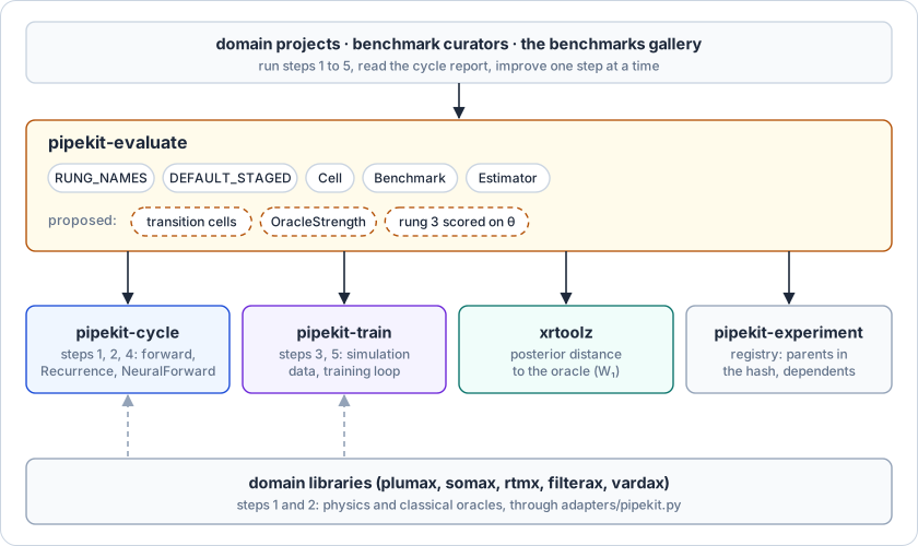
Figure 1:The ladder in pipekit-evaluate is the cycle; the steps run where their computation lives.
pipekit-evaluate owns the cycle’s vocabulary (rungs, levels, transitions, oracle strength), the reference rule and the runner. Today it imports pipekit-cycle only through an optional extra (
cycle), and it would import pipekit-experiment and xrtoolz the same way.pipekit-cycle owns steps 1, 2 and 4 as operators: the forward model (
CallableForward,NeuralForward), the iterative inversion (Recurrence) and the assimilation cycles (DACycle). It never imports pipekit-evaluate.pipekit-train owns steps 3 and 5, which are the training data drawn from the step-1 simulator (
SimulationDataset) and the training loop. It never parses a contract or a cell.
xrtoolz holds the distance from a posterior to the oracle’s (workstream C), and pipekit-experiment holds the lineage inside the hash (workstream B). The domain libraries (plumax, somax, radtrax for step 1; filterax, vardax, pyrox for step 2) hold the physics and the classical oracles, which we reach through adapters/pipekit.py. Otherwise, neighbours follow the stack rules.
The running example: one retrieval, six steps¶
The problem. We retrieve a methane column enhancement from a multiband sensor, and we take the retrieval through all six steps of the cycle, which is the cell of the matrix that the scoping report works through in its section 4.1. The sensor is the one of Reports 10 and 11, so their results carry over.
The data. A sensor measures transmittances in bands, indexed by . The retrieved quantity is the column enhancement , a scalar physical quantity (the ladder calls it θ, as in known_theta), and holds the band absorption coefficients, . With the noise , the generative model is (1) to (4):
where is the forward model with band components , and is the observation-error covariance with . We work in covariances throughout this page, so every weight below is an inverse covariance. The test set is scenes drawn from the prior with seeds of their own, disjoint from every training set below. This is the L1 → L2 row, so structured observations (transmittances) go in and a retrieved geophysical variable () comes out.
What exists. Every step runs on the pinned code except where a line is marked user (markers). The ladder’s task, estimates and scorers are user code, as in Report 14, and the polynomial emulator and the Gaussian head are small least-squares fits, so the whole cycle runs in under a minute and every number is checkable. Report 11 trains an amortized retrieval for the same sensor with Equinox through pipekit-train (its stage 6), and the cycle does not depend on which kind of model fills a step.
Stage 1 · The simple model, as a ladder task (pipekit-cycle → pipekit-evaluate)¶
TL;DR. Write the forward model as a pipekit-cycle operator and the retrieval as a ladder task, and read the rule the ladder already applies to each step.
Problem. A ladder Task bundles a prior, the step-1 simulator, an observation operator and the data each rung is scored against, which are the known for the oracle, the simulator’s outputs for the emulator, and the observations that every estimator receives.
1 2 3 4 5 6 7 8 9 10 11 12 13 14 15 16 17 18 19 20# Shapes: B = 5 bands; N = 500 test scenes import pipekit_cycle as pc from pipekit_evaluate.benchmark import (DEFAULT_STAGED, LEVEL_NAMES, RUNG_NAMES, Cell, Task) # h_b(α) = exp(−k_b α) forward = pc.CallableForward(lambda a, dt: np.exp(-K * a), dt=1.0) # (,) → (B,) today task = RetrievalTask() # prior 𝒰(0, 300), simulator, obs user isinstance(task, Task) # → True today task.datasets() # α (N,), h(α) (N, B), y (N, B) user RUNG_NAMES # {1: simple_model, 2: model_based_inference, # 3: emulator, 4: emulator_based_inference, # 5: amortized_predictor, 6: improve} today DEFAULT_STAGED # {1: none, 2: known_theta, 3: simulator_output, # 4: oracle_posterior, 5: oracle_posterior, # 6: best_validated_below} today LEVEL_NAMES["L2"] # → "gap_filled_obs" today Cell("L2", rung=4).label # → "L2/r4/c0": not "L1 → L2" today
The step-1 model and the task, and the rule the ladder applies to each rung, from a real run.
The six steps are the ladder’s six rungs, and its default rule is the cycle’s: the oracle (rung 2) is scored against the known truth, the emulator (rung 3) against the simulator it replaces, and both fast inversions (rungs 4 and 5) against the oracle’s posterior. However, two things do not fit the cycle matrix. 1) A cell names one level, so the L1 → L2 retrieval, the L2 → L3 gap filling and the L3 → L4 forecast cannot be told apart once two rows share an output level. 2) The ladder names L2 “gap_filled_obs” while its own design note describes it as “per-pixel geophysical retrievals (gaps allowed)”, which is what the overview’s levels call L2 (workstream A1).
Stage 2 · The oracle, and a cheaper inversion below it (pipekit-cycle)¶
TL;DR. Compute the exact posterior for every scene, check it against the truth, and compare it with a Gauss–Newton fit one step down the complexity axis.
Problem. With the flat prior of (4), the posterior is
The oracle evaluates it on = 30,001 nodes over [0, 300], with a step of 0.01 against a smallest posterior standard deviation of 0.068, so it is exact to quadrature. A scale to compare it with is the local Fisher information. With the Jacobian of the forward model, whose entries are , the width is the Cramér–Rao bound for an unbiased estimator at . However, it is not a bound on the oracle, which is a posterior mean that uses the prior and is biased near the boundary . The Laplace step below the oracle fits by Gauss–Newton on the cost , and it reports the width , which is the square root of at .
1 2 3 4 5 6 7 8 9 10 11 12 13 14 15 16 17# Shapes: N = 500 scenes; N_g = 30,001 nodes; B = 5 # log p(α_g | y) = −½ ‖y − h(α_g)‖² / σ_ε² + c # w_g ∝ ω_g p(α_g | y), ω trapezoidal (½ at α = 0 and 300), ∑_g w_g = 1 oracle = grid_posterior(y, f) # (N, B) → (N, N_g) user # α ← α + J_hᵀ(y − h(α)) / (J_hᵀ J_h) until |Δα| < 10⁻⁸ gn = pc.Recurrence( GaussNewtonStep(y), # user condition_op=Lambda(lambda s: s.residual_norm < 1e-8), max_iters=50) # (N,) → (N,) today a_hat, _ = gn(a0, pc.IterationState()) # today # σ_L = σ_ε / ‖J_h(α̂)‖ J = K * f(a_hat) # (N, B): |∂h_b/∂α| laplace = GaussEstimate(a_hat, SIG / np.linalg.norm(J, axis=1)) # (N,) user # RMSE vs α: oracle 0.236, Laplace 0.237; RMS of σ_ε / ‖J_h(α)‖ 0.247 # 95 % coverage vs α: oracle 0.962, Laplace 0.960 (s.e. 0.010) # Laplace mean within 0.26 oracle widths of the oracle's, every scene
The oracle by quadrature and the Laplace step as a Recurrence, scored against the truth, from a real run.
The oracle covers the truth at the nominal rate, and its error is of the size that the local Fisher information sets (a little below it, 0.236 against 0.247, because the prior and the boundary help). So on this problem step 2 is an oracle in the strong sense: the forward model is known and the posterior is computed, not approximated. The Laplace step agrees with it to a quarter of a standard deviation everywhere, which is the complexity axis doing its job, as a richer inversion must first reproduce the simpler one where both are valid.
Stage 3 · Two emulators of the forward model (pipekit-train → numpy)¶
TL;DR. Fit two polynomial emulators to simulations of the forward model and score them against the simulator, the reference rung 3 calls for.
Problem. An emulator of degree writes each band as a polynomial in , with coefficients fitted on the training split of a SimulationDataset of 2,000 seeded draws, (6):
where the monomials of a draw are
with , so the emulator is .
1 2 3 4 5 6 7 8 9 10 11# Shapes: 1,600 training draws; B = 5; C (d + 1, B) sim = pt.SimulationDataset(forward, PriorDraw(), n_samples=2000, seed=0) # today len(sim) # → 1600: the train split today # C⋆ = argmin_C ‖V C − H‖², V (1600, d + 1) and H (1600, B) stack the v(α_n)ᵀ and h(α_n)ᵀ C4 = fit_emulator(4) # (1600, 5) → (5, B) user C6 = fit_emulator(6) # (1600, 7) → (7, B) user # max_b,α |ĥ_b(α) − h_b(α)| / σ_ε over 3,001 values of α # degree 4: 2.2 σ_ε (3.2 % of the transmittance at worst) # degree 6: 0.03 σ_ε # on the 500 test scenes only: degree 4, 2.01 σ_ε (stage 6's figure)
Training data from the step-1 simulator, two emulators, and their error against the simulator, from a real run.
Judged as a forward model, the degree-4 emulator looks good, as its worst error is 3.2 % of the transmittance. However, judged in the unit that the problem fixes (the noise ), it is off, and the next stage shows what that costs. This is the scoping report’s claim about benchmarks made concrete: the tolerance in a step-3 contract cannot be written until one knows the noise of the step-4 problem, so writing it down is the act of understanding it.
Stage 4 · The oracle’s inversion, rerun with each emulator (pipekit-cycle → xrtoolz)¶
TL;DR. Rerun the oracle’s quadrature with each emulator in place of the simulator and score the result against the oracle’s posterior.
Problem. Step 4 replaces with in (5). With the distribution functions of the step-4 and oracle posteriors, the 1-Wasserstein distance (8)
is zero only when the two posteriors agree. We report in units of the oracle’s posterior standard deviation , so it reads as “how many widths apart”.
1 2 3 4 5 6 7 8 9 10 11 12 13# Shapes: N = 500 scenes; N_g = 30,001 nodes; 2,000 draws per scene fast = grid_posterior(y, f_hat_4) # (N, B) → (N, N_g) user # (μ̂_α|y − μ_α|y) / σ_α|y, the mean shift in oracle widths # degree 4: RMS 0.44, max 1.94; width ratio 1.00; W₁ / σ_α|y 0.37 # degree 6: max 0.02 # 95 % coverage vs α: degree 4 0.948, degree 6 0.962 (the oracle's) # W₁ = ∫ |F̂ − F| dx, from 2,000 samples of each, in oracle widths a = xr.DataArray(fast.sample(2000, key=1), dims=("scene", "member")) b = xr.DataArray(oracle.sample(2000, key=2), dims=("scene", "member")) w1 = xrtoolz.metrics.wasserstein_1(a, b) # (N, 2000) → (N,) today (w1 / oracle.sd()).mean() # (N,) → () : 0.37 # the oracle against itself, over 20 key pairs: 0.040 ± 0.0004 # degree 6 on the same pairs: 0.041, inside that null; exact W₁ / σ_α|y 0.004
Emulator-based inference against the oracle, exactly and through xrtoolz, from a real run.
A 3 % emulator moves the posterior mean by up to 1.9 widths, while the width of the posterior does not change at all and the coverage of the truth only drops from 96.2 % to 94.8 %. On the same 500 scenes, the paired difference (11 scenes lost, 4 gained) is −1.4 ± 0.8 points, z = −1.8, so a check against the truth at this sample size would not reject it at 95 %, and a check on the uncertainty alone would pass outright. The degree-6 emulator, at , reproduces the oracle to 0.02 widths. So scoring step 4 against the oracle, as the ladder’s rule does, is what makes this visible, whereas scored against the truth alone the degree-4 inversion looks like a good retrieval. xrtoolz’s wasserstein_1 reproduces the exact , but it only takes samples, so an exact posterior on nodes must be sampled first. Two samples of one posterior are never 0 apart, so the sample estimate is biased upward. Over 20 independent pairs of 2,000 draws, the oracle against itself scores 0.040 widths (standard deviation 0.0004, largest 0.041). The degree-6 emulator scores 0.041 on the same pairs, which is inside that spread, so the sample estimate cannot tell it from the oracle, whereas the exact is 0.004 (workstream C1).
Stage 5 · An amortized predictor, against the truth and the oracle (numpy → xrtoolz)¶
TL;DR. Fit one Gaussian predictor for every spectrum, and see that scoring it against the truth and scoring it against the oracle give different verdicts.
Problem. The predictor is , with the mean and the log-variance both linear in the features , which we build from the per-band inversions . Both are fitted once, by least squares on 20,000 simulated pairs drawn from (1) to (4), as (9) and (10):
with the encoder parameters and the residuals . The predictor then sets and , since . A predictor calibrated against the truth has for the standardised error .
1 2 3 4 5 6 7 8 9 10# Shapes: 20,000 training pairs; φ(y) (N, 8); N = 500 test scenes # φ(y) = [1, α̂₁ … α̂₅, ᾱ², ᾱ³] on the scale α / 300, ᾱ the band mean of α̂_b # μ_q = φᵀν_μ, log σ_q² = φᵀν_σ + 1.27 q = amortized(y) # (N, B) → μ_q (N,), σ_q (N,) user # against α: RMSE 0.255; 𝔼[ζ²] 0.90 (s.e. 0.063); 95 % coverage 0.954 # against the oracle: width ratio 1.16; 1.53 for α < 50 (83 scenes) # mean shift for α < 50: 1.04 widths RMS, 3.6 at worst # W₁ / σ_α|y 0.38, over the real line: the Gaussian's tails outside [0, 300] # are added in closed form, σ_q (ζ₀ Φ(ζ₀) + 𝒩(ζ₀; 0, 1)) on each side, # with ζ₀ the boundary in standardised units
The amortized Gaussian head, scored two ways, from a real run.
Against the truth, the predictor passes, with (within 1.6 standard errors of 1) and 95.4 % coverage. However, against the oracle it is a different estimator. Where the column is small and the posterior narrow, its mean is noisier than the oracle’s (1.04 widths off), and it widens its intervals by 53 % to stay honest about that. The truth only checks that the predictor knows how wrong it is on average over the prior, whereas the oracle checks that it reproduces the posterior scene by scene, which is the question an amortized predictor must answer. The ladder scores rung 5 against the oracle only, so today the two verdicts need two runs (Report 14’s A4, gate C2 here).
Stage 6 · The ladder and the lineage (pipekit-evaluate → pipekit-experiment)¶
TL;DR. Run every rung through the shipped ladder, store every artifact in the registry with its parents, improve the emulator, and ask what must be rerun.
Problem. (a) The ladder. Five estimators fill five cells at level L2: Laplace (rung 2, complexity 0), the quadrature oracle (rung 2, complexity 1), the degree-4 emulator (rung 3), its inversion (rung 4) and the amortized head (rung 5). (b) The lineage. Step 6 replaces the degree-4 emulator with the degree-6 one. An artifact is stale when it was built from the old emulator, either directly or through another artifact, so the set of stale artifacts is the set of descendants of the old emulator in the graph of parents.
1 2 3 4 5 6 7 8 9 10 11 12 13 14 15 16 17 18 19 20 21 22 23 24 25 26 27 28 29 30 31 32 33 34 35# Shapes: N = 500; spectra (N, B) in σ_ε; posteriors in oracle widths report = pe.Benchmark(task=task, scorers=[Score()], level="L2", estimators=[ Rung(2, 0, laplace), # y ↦ Laplace estimate Rung(2, 1, lambda y: grid_posterior(y, f)), # the oracle EmulatorRung(3, 0, f_hat_4), Rung(4, 0, lambda y: grid_posterior(y, f_hat_4)), # step 4 Rung(5, 0, amortized)]).run() # Rung, EmulatorRung: user today # L2/r2/c0 known_theta max |α̂ − α| 1.12, RMSE 0.237 # L2/r2/c1 known_theta max |α̂ − α| 1.12, RMSE 0.236 # L2/r3/c0 simulator_output max |ĥ − h| 2.01 σ_ε, RMSE 0.277 σ_ε # L2/r4/c0 oracle_posterior max shift 1.94, width ratio 1.00 # L2/r5/c0 oracle_posterior max shift 3.63, width ratio 1.16 EmulatorRung.fit(task) # reads α: rung 3 needs α, not y user reg = px.LocalModelRegistry(root) # today h0 = reg.store(Artifact("prior", {"low": 0, "high": 300}), tags={"rung": 1, "role": "prior"}) # today h1 = reg.store(Artifact("simulator", {...}), tags={"rung": 1}) # today h2 = reg.store(Artifact("grid_posterior", {"nodes": 30001, "low": 0, "high": 300, "rule": "trapezoid"}, parents=[h0, h1]), tags={"rung": 2, "role": "oracle"}) # today # another prior support → another oracle hash (asserted); another # calibration constant → another head hash (asserted) h3 = reg.store(Artifact("poly_emulator", {...}, parents=[h1]), tags={"rung": 3, "oracle": h1}) # today # … rungs 4 and 5 likewise (parents [h0, h3] and [h0, h1]; rung 5's # config holds ν_μ, ν_σ and the calibration constant −1.27); then step 6 # → new hashes for rungs 3 and 4; rung 5's unchanged (parents h0, h1) dependents(h3) # → [old rung 4]: a scan of configs user reg.store(emulator_6, tags={"oracle": "x"}) # → the same hash; its oracle tag is now "x" today reg.list(tags={"parents": [h1]}) # → []: parents are config, not tags today
The cycle through the shipped runner and registry, from a real run.
One Benchmark.run() call scores rungs 2 to 5 and resolves the reference of each rung as stage 1 read it. Step 1 is the task built before the call, and step 6 happens outside it, as the notebook stores the new emulator and calls the runner again. After the improvement, rerunning it changes the rung-3 and rung-4 rows (to and a 0.02-width shift) and leaves rung 5’s unchanged, because rung 5 was trained on the simulator. However, three things needed glue. 1) Rung 3 is a forward emulator, a map from to , but the runner calls every estimator on the observations, so the emulator reads from the task inside fit (workstream A3). 2) The registry can carry lineage in two ways, and neither is enough. Tags are outside the hash, so storing the same emulator again with another oracle tag silently replaces it, and a tag filter matches whole values, so it cannot ask which artifacts list a given parent. Parents in the configuration are hashed, which is right (and which is why a new emulator gave rung 4 a new hash), but nothing indexes them, so “what depends on this?” is a scan of every stored configuration (workstream B). 3) A configuration that holds a mapping cannot be loaded back, as from_state refuses non-primitive values (pipekit/_base/operator.py:251).
The scoping report’s names, checked¶
Table 1 sets every name that the scoping report uses against the pinned code.
Table 1:Every name the scoping report uses, against the pinned code.
| Scoping report | At the pinned revisions |
|---|---|
| the six steps; step 2 as oracle | RUNG_NAMES and DEFAULT_STAGED in pipekit_evaluate.benchmark (stage 1) |
CycleStageBenchmark(target_step, oracle_step, l_transition, oracle_artifact_hash, oracle_strength) | does not exist; Cell(level, rung, complexity) and ReferenceRule cover the step and its reference; transition, oracle hash and strength are new (A1, A2) |
CycleBenchmark.run_full_cycle | does not exist; Benchmark(...).run() scores rungs 2 to 5 in one call, while step 1 (the task) and step 6 (store an improvement, rerun) stay outside it (stage 6) |
OracleStrength | does not exist; ReferenceSource says where a reference comes from, not how far to trust it |
ModelRole, ArtifactLineage | do not exist; LocalModelRegistry.store(..., tags=) stores free tags outside the hash (stage 6) |
pc.DACycle(forward_model, obs_op, analysis_step, n_steps) | exists, with obs_source and save_history as well (da.py:84) |
pc.NeuralForward(model_op, dt) | exists (forward.py:136) |
pc.Recurrence for iterative retrieval | exists (cycle.py:265); stage 2 runs Gauss–Newton with it |
pt.SimulationDataset(forward_model, prior, n_samples), pt.CachedDataset(source, cache_dir) | exist (dataset.py:228, :393) |
pt.TrainingLoop(..., n_epochs=, backend="lightning") | TrainingLoop counts max_steps, not epochs; the Lightning backend raises NotImplementedError (Report 11) |
pt.MSE, pt.NLL | exist (loss.py) |
pa.ModelOp | no such alias; the Equinox adapter’s EquinoxModelOp or pipekit-jax’s JaxModelOp |
px.S3ModelRegistry | exists (registry.py) |
pe.MultiTrackEvaluation, EvaluationReport.diff | do not exist; Report 15 drops the first, Report 14 proposes the report (A3) |
geotoolz.matched_filter.CH4MatchedFilter | MatchedFilter, MatchedFilterPixel, MatchedFilterSNR exist; no CH₄-specific class |
| BAEMR retrieval | not identified; the gallery found the same |
plumax.PlumeForward, ColumnObs, filterx…EnKFAnalysis, pyrox_nn…ConditionalNormalizingFlow, RTMX.RTM | not pinned in references/, so not checked; the scoping report’s filterx is filterax |
| “the 23 benchmarks” of the gallery | 18 entries; 23 contracts once entry 5.1 is split into its six (gallery) |
Current-state audit¶
Four of the eight symbol groups need action (Table 2), and Figure 2 shows what the sketches on this page call. We read them on 14 October 2026 at the revisions in the report’s header, on main of each submodule.
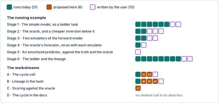
Figure 2:Of the page’s 40 marked stack calls, 21 run today, 6 are proposed by this report’s workstreams and 13 are code the reader writes (how to read it: conventions).
Table 2:The cycle’s surface, by symbol group.
| Symbols | Defined in | Used by | Verdict |
|---|---|---|---|
RUNG_NAMES, LEVEL_NAMES, Cell | pipekit-evaluate benchmark/cube.py | Benchmark, Reports 14 and 15 | Split ownership. A cell names one level, not a transition; L2 is named gap_filled_obs but described as retrievals (cube.py:28) |
DEFAULT_STAGED, DEFAULT_COMPLEXITY, ReferenceRule, ReferenceSource | benchmark/reference.py | Benchmark | Healthy. The cycle’s oracle rule, as data a domain can override; no notion of how strong the oracle is |
Benchmark, CellResult | benchmark/run.py | stage 6 | Split ownership. Every estimator is called on the observations (run.py:108), so rung 3 needs glue; one reference per cell (Report 14) |
Estimator, Estimate, Task, Oracle | benchmark/protocols.py | stage 6 | Healthy. Enough for every rung once rung 3 is called on ; Oracle is still not consumed (Report 14) |
CallableForward, NeuralForward, Recurrence, DACycle | pipekit-cycle forward.py, cycle.py, da.py | stages 1, 2 and 6; Reports 10 and 11 | Healthy. Steps 1, 2 and 4 as operators; an emulator drops in through NeuralForward |
SimulationDataset, TrainingLoop | pipekit-train dataset.py, loop.py | stage 3; Report 11 | Healthy for steps 3 and 5; the dataset hash ignores the forward model (Report 11’s A3), so it cannot name step 1 as a parent |
LocalModelRegistry.store, list, tag | pipekit-experiment registry.py:113, :180 | stage 6; Report 12 | Split ownership. Tags are outside the hash and merged on re-store (:159); list matches whole tag values (:195); no reverse lookup |
wasserstein_1, Wasserstein1 | xrtoolz metrics/_src/distributional.py:144 | stage 4 | Healthy. Samples only: no weights, so a posterior on nodes is resampled, and the sample estimate is biased upward by about 0.04 widths at 2,000 draws |
Smaller findings:
A dictionary in an operator’s configuration does not reload.
Operator.from_staterefuses non-primitive configuration values (pipekit/_base/operator.py:251), so an artifact whose configuration nests its settings stores fine but cannot be loaded back (stage 6). Flat keys or a JSON string work.Skipping step 3 needs nothing. A run with no rung-3 estimator simply has no rung-3 row, and a run with no rung-2 estimator reports “no oracle (rung-2) estimator available” on rungs 4 and 5 (
run.py), which is the honest answer. So the code already answers the scoping report’s open question 3.The ladder’s design note already plans the cycle report. Its build order ends in “the level × rung × complexity
BenchmarkReport+ DVC wiring”, and it names the plume pilot as the first slice because “every rung already exists” (benchmark_ladder.md§7).
Workstream A · The cycle cell¶
Decision. A cell of the cycle matrix is a ladder cell with a transition, and a contract names its oracle and how far to trust it. Nothing else about the ladder changes (Table 3).
Table 3:Workstream A’s moves.
| Symbol | Destination | Reason |
|---|---|---|
Cell(level, rung, complexity, source=None) with label "L1→L2/r4/c0" | benchmark/cube.py | stage 1: one level cannot tell retrieval, gap filling and forecasting apart |
LEVEL_NAMES["L2"] = "retrieved_obs" | benchmark/cube.py | the ladder’s own description of L2, and the overview’s |
OracleStrength (physics_derived, classical_method, human_labels, heuristic) | benchmark/reference.py, beside ReferenceSource | the scoping report’s strong and weak oracles; the reference rule says where, not how far to trust |
oracle: {artifact, strength} on BenchmarkContract; strength on each CellResult scored against it | Report 15’s contract; benchmark/run.py | a report row says what its reference was worth; a heuristic or human_labels oracle warns and still scores |
rung 3 called on task.datasets()[truth_key] | Benchmark.run | stage 6: a forward emulator maps to ; the fit workaround goes |
A1 · Transition cells¶
A cell gains an optional source level, so that a contract’s task (Report 15’s "L1->L2") and its cell use one vocabulary, and a cell without one is read as it is today. We rename the ladder’s L2 to match its description. Report 15 and the gallery use “L1 → L2” for gap filling, which on the renamed levels is L2 → L3, and that relabelling is an open question below, not a silent change.
A2 · Oracle strength¶
A contract names its oracle by artifact hash and strength. The runner copies the strength onto every row it scores against that oracle, and it warns, without refusing, when the strength is human_labels or heuristic. The scoping report leans the same way (its open question 1).
A3 · The emulator rung¶
Benchmark passes the truth, not the observations, to a rung-3 estimator, and scores it against the simulator’s outputs as it does today.
1 2 3 4 5 6 7 8 9 10# Shapes: α (N,); h(α) (N, B) # Today: EmulatorRung.fit(task) # stores α itself user pe.Benchmark(task, estimators, scorers, level="L2").run() # today # → "L2/r3/c0", ref simulator_output; no strength on any row # After: pe.Benchmark.from_contract(c, estimators=[...]).run() # → "L1→L2/r3/c0": ĥ(α) against h(α), 2.01 σ_ε proposed (A1, A3) # c.oracle = {"artifact": h2, "strength": "physics_derived"} # → rows r4 and r5 carry "physics_derived" proposed (A2)
The emulator rung and an oracle with a strength, before and after workstream A.
Workstream B · Lineage in the hash¶
Decision. An artifact’s parents are part of what the registry hashes, and the registry answers which artifacts descend from a given one (Table 4).
Table 4:Workstream B’s moves.
| Symbol | Destination | Reason |
|---|---|---|
store(op, *, parents=(), ...) writing lineage.json into the hashed payload | pipekit_experiment.registry | stage 6: a tag can be replaced without changing the hash |
ArtifactLineage(parents, oracle, training_artifact) | pipekit_experiment.artifacts, beside TrainingArtifact | the scoping report’s record, minus the benchmark results, which point the other way (a report names the model, Report 15’s E2) |
dependents(hash), descendants(hash) | ModelRegistry protocol and both registries | stage 6: “what must be rerun?” is a scan today |
a rung tag ({"rung": 3}) by convention | the ladder’s docs | the role the scoping report’s ModelRole would carry; list(tags=) filters it today |
B1 · Parents in the payload¶
The hash of a stored artifact covers its operator state, its weights and its lineage record. So two artifacts with the same weights and different parents are different artifacts, and nothing can rewrite a parent after the fact. TrainingArtifact.dataset_hash becomes one parent among others, and Report 11’s A3 (the simulator in the dataset hash) is what makes that parent trustworthy.
B2 · Dependents¶
The registry keeps a reverse index from parent to child, which it writes at store time, so descendants(h) is the stale set when h is replaced.
1 2 3 4 5 6 7 8 9 10 11# Shapes: hashes of 64 hex characters # Today: reg.store(emu_6, tags={"oracle": h1}) reg.store(emu_6, tags={"oracle": "x"}) # → the same hash; the oracle tag is now "x" today dependents(h3) # scan every operator.json user # After: h3 = reg.store(emu_4, parents=[h1]) # proposed (B1) reg.store(emu_4, parents=[h_other]) != h3 # proposed (B1) reg.descendants(h3) # → [h4]; rung 5 has parent h1 # proposed (B2)
Asking what an improvement makes stale, before and after workstream B.
Workstream C · Scoring against the oracle¶
Decision. The distance from a posterior to the oracle’s is an xrtoolz metric that takes weights, and the amortized rung is scored against the oracle and the truth in one run (Table 5).
Table 5:Workstream C’s moves.
| Symbol | Destination | Reason |
|---|---|---|
wasserstein_1(a, b, *, weights_a=None, weights_b=None, ...) | xrtoolz.metrics | stage 4: an exact posterior on nodes is resampled today, and the estimate’s upward bias (the oracle against itself scores 0.040 ± 0.0004 widths at 2,000 draws) hides the degree-6 emulator’s exact 0.004 |
two references for rung 5 (oracle_posterior and known_theta) | Report 14’s A4 in benchmark/run.py | stage 5: the truth says “calibrated”, the oracle says “53 % too wide where is small”; both belong on the row |
1 2 3 4 5# Shapes: nodes (N_g,); weights (N, N_g) # W₁ = ∫ |F̂ − F| dx xrtoolz.metrics.wasserstein_1( nodes, nodes, weights_a=fast.w, weights_b=oracle.w) # (N, N_g) → (N,); 0.37 σ_α|y proposed (C1)
Distance to the oracle with weights, after workstream C.
Workstream D · The cycle in the docs¶
Decision. The overview states the shipped oracle rule, and the reports that already ran steps of the cycle say which ones. Both changes land with this page.
Correct the overview’s rule (D1). The overview said every cell “uses the column before it as its oracle”, whereas the shipped rule scores the emulator against the simulator and both fast inversions against step 2. This change corrects the sentence, and it replaces the overview’s planned
ModelRole,ArtifactLineageandCycleStageBenchmarkwith workstreams A and B.Link the reports to the steps (D2). Report 11’s stage 2 is step 3 of a forecast row (its stage 3 runs that emulator forward, which is a forecast and not an inversion), and its stages 6 and 7 are steps 5 and 2 of this retrieval. Report 14’s stage 4 fills rungs 2 and 5, and Report 15’s contract is what each cell is benchmarked by. This change adds one sentence to each report that points here, because the scoping report’s 30 to 80 lines per report would repeat this page.
Testing gates¶
Each workstream merges only when its gates (Table 6) pass on the running example.
Table 6:Gates, by workstream.
| Gate | Workstream | Passes when |
|---|---|---|
| A1 Transition cell | A | Cell("L2", 4, source="L1").label == "L1→L2/r4/c0", a cell without a source keeps today’s label, and LEVEL_NAMES["L2"] == "retrieved_obs" |
| A2 Oracle strength | A | stage 6’s rows for rungs 4 and 5 carry physics_derived; with a heuristic oracle the same run emits one UserWarning and reproduces the same scores |
| A3 Emulator rung | A | stage 6’s rung-3 estimator, with no fit workaround, scores (degree 4) and (degree 6) against the simulator |
| B1 Lineage hash | B | storing the stage-6 emulator with another parent gives another hash, and with the same parent and other tags the same hash |
| B2 Dependents | B | after stage 6’s improvement, descendants(h3) is exactly the old rung-4 artifact, and the rung-5 artifact appears in no descendant set of an emulator |
| C1 Weighted W₁ | C | with weights, wasserstein_1 reproduces stage 4’s exact (0.37 for degree 4, 0.004 for degree 6) to 10⁻³, and is 0 for a posterior against itself |
| C2 Two references | C | one run reports rung 5’s width ratio against the oracle (1.16) and its against the truth (0.90) on the same row |
| D1 Docs | D | the overview’s oracle sentence matches DEFAULT_STAGED, and myst build --html reports no warnings |
| D2 Links | D | Reports 11, 14 and 15 each link to this page (its running example, stage 6 and workstream A), and every link resolves in myst build |
Sequencing and risks¶
We start with the docs and the vocabulary, because they cost nothing and every later change uses them, then lineage and scoring, and then a real cycle (Figure 3).
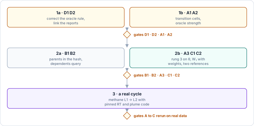
Figure 3:Name the cycle, then record its lineage and score it, then run it on real data.
The oracle is expensive to keep. Step 2 has to stay runnable on new data to score new submissions. Fallback: run it on a fixed, versioned validation set and at a lower cadence than production, and record the set’s hash in the contract, so its cost is paid once per oracle version.
Many artifacts per row. There are five steps per transition and five transitions per domain. Fallback: the registry already content-addresses each one, and the lineage graph is a chain per row with few cross-links, so the dependents index stays small.
Weak oracles. In data-first cycles, step 2 is a supervised baseline on uncertain labels, and matching it is not the same as being right. Fallback: the oracle’s strength is on every row (A2), and the physical-constraint scorers of Report 14 are mandatory for rungs scored against a weak oracle.
Exact oracles are rare. Stage 2’s posterior is exact because is one number. For a field or a plume, step 2 is an EnKF, a 4D-Var or MCMC. Fallback: the complexity axis (MAP below Laplace below NUTS) validates the oracle itself before it validates anything else, as stage 2 does with Laplace.
The physics libraries are not pinned. plumax, radtrax, filterax and vardax are named but are not in
references/, so the real methane cycle cannot run here yet. Fallback: phase 3 waits for them, whereas phases 1 and 2 only need the pinned packages.
Open questions¶
Which levels do gap filling and retrieval connect? The ladder (and Report 15 and the gallery, which follow it) calls gap filling L1 → L2, whereas the overview’s levels and the scoping report’s matrix call retrieval L1 → L2 and gap filling L2 → L3. Recommended: the overview’s levels, with the tasks of Report 15 and the gallery relabelled in one change. Alternative: keep the ladder’s levels and rename the overview’s.
Does an oracle’s strength propagate? The scoping report scores its direct predictor against step 4 (its section 6.3), and a domain may override the default rule that way to save oracle runs, but that reference carries step 4’s emulator error. Should such a row record the weaker of the two strengths?
Entering mid-cycle. A team that is handed a trained emulator without its simulator can run steps 4 and 5 with the emulator as the reference. Is that a
heuristicstrength with no step-1 parent, or a strength of its own?Cross-domain cycles. Methane retrieval feeding ocean carbon assimilation chains two rows. Is that the gallery’s cascade contract (entry 5.1), with one cycle per row?
When does pipekit-jax matter? Step 4 with a differentiable emulator enables gradient-based inversions, which the quadrature of stage 4 does not need. Should the first real cycle use one, to settle pipekit-jax’s timing?
Upcoming work¶
Table 7 lists the follow-ups outside the workstreams.
Table 7:Follow-ups from checking the scoping report against the code.
| Item | Where | Why |
|---|---|---|
| Map each gallery entry to its cells (transition, steps present, oracle strength) | benchmarks gallery | the scoping report’s appendix; needs open question 1 settled first |
| Pin plumax, radtrax, filterax and vardax | references/, UPSTREAM | the real methane cycle and the scoping report’s step-1 and step-2 names cannot be checked otherwise |
| Flat configurations for stored artifacts | pipekit Operator.from_state or the registry’s docs | stage 6: a nested configuration stores but does not reload |
| The plume pilot as the first real cycle | pipekit-evaluate docs/design/plume_pilot.md | the ladder’s design note picks it because every rung exists |
References¶
Sources¶
The scoping report (numbered 16 in its draft, 17 here), “Report 16 — The data-driven modeling cycle and benchmark-gated L0–L4 refinement” Johnson, 2026, and the gallery draft it extends Johnson, 2026.
The pinned code in
references/: pipekit-evaluate (benchmark/anddocs/design/benchmark_ladder.md), pipekit-cycle (forward.py,cycle.py,da.py), pipekit-train (dataset.py,loop.py), pipekit-experiment (registry.py,artifacts.py), pipekit (_base/operator.py), xrtoolz (metrics/_src/distributional.py) and geotoolz (matched_filter/).The running example’s notebook, described in Section ??.
- Johnson, J. E. (2026). Report 16 — The Data-Driven Modeling Cycle and Benchmark-Gated L0–L4 Refinement. Unpublished scoping report.
- Johnson, J. E. (2026). Benchmarks Gallery. Unpublished draft, companion to the Report 15 scoping report.