pipekit-evaluate
Report 14 · Multidimensional evaluation, checked against what the stack already scores
Abstract¶
A single RMSE cannot tell a correctly shaped but displaced methane plume from a featureless field, it cannot see that a forecast has lost its small scales, and it cannot score whether the right plumes were detected. The scoping report names these failures, organises evaluation along three axes (the Unit scored, the Lens of critique and the lifecycle Stage) and proposes pipekit-evaluate to own every metric. However, the pinned code tells a different story. pipekit-evaluate 0.0.2 ships a benchmark ladder (levels, rungs, an oracle rule and a runner), and it calls the Unit × Lens × Stage taxonomy “still planned”. Meanwhile, xrtoolz.metrics already ships most of the matrix which the scoping report marks as missing: spectral skill, SSIM, phase-shift error, instance matching, geostrophic-balance and budget residuals, and wrappers by lead time, region and frequency band. The capability index hid this, because it only lists four xrtoolz names. This report keeps the framework, places each missing metric in the library that already reserves its name, and gives pipekit-evaluate the taxonomy tags, the report artifact and the ladder. Every number below is from a real run.
About this report
| Status | Partly built. Originally a two-part scoping proposal (“committed”: a framework and a package); the framework is kept, the package’s scope is redrawn around what ships |
| Reading time | about 35 minutes |
| Audience | anyone scoring a model, a retrieval or a forecast with the stack, or designing a benchmark |
| Companions | Report 13 (forecast verification, which this extends); Report 10, Report 11, Report 12 (the cycle, training and registry this connects to); Report 9 (use cases); Report 16 (the stack rules); Report 17 (the ladder vocabulary) |
| Code checked against | pipekit-evaluate 0.0.2 at pipekit ef3c17f; xrtoolz 0.0.5 at 308c7f2; geotoolz 0.10.2 with geocatalog at 088475e. pipekit-evaluate’s 18 tests pass. Read on 13 October 2026 |
| Running example | every output is from one run of notebooks/reports/report14_pipekit_evaluate.py (the metrics of stages 1 to 3 and the ladder of stage 4), which seeds every field and asserts each number the page shows |
| Design docs | pipekit-evaluate’s benchmark_ladder.md and four pilots (ocean, plume, land extremes, fusion), all “design only, no code” |
Summary¶
Decision. Metrics live with their carriers: xrtoolz.metrics for xarray fields, statistics, events and physical checks, geotoolz for GeoTensor detection building blocks, and pipekit-train for differentiable losses. pipekit-evaluate owns what no carrier library can, which is the taxonomy as tags on scorers, a scorer adapter over any metric operator, the evaluation report, and the benchmark ladder it already ships. There is no pipekit-array.metrics.classification and no third catalog type.
A. The taxonomy and the report in pipekit-evaluate. We tag every
Scorerwith its unit, lens, stages and differentiability (A1), adapt any xrtoolz metric operator into aScorer(A2), growBenchmarkReportinto anEvaluationReportwhich can be hashed, filtered, diffed and turned into a table (A3), and fix the ladder’s rough edges (A4).B. The missing metrics, where their names are reserved. FSS and a shift-blind spectrum comparison (B1), POD, FAR, CSI and the contingency table, whose names
xrtoolz.metrics.objectalready reserves (B2), NSE, the index of agreement, Brier and the multivariate energy score (B3), and the Hausdorff distance and structure functions (B4).C. The missing wrappers. By season or month (C1), by event (C2) and by member (C3), beside the shipped lead-time, region and band wrappers.
D. The trajectory unit. Particle advection, dispersion and FTLE in a new
xrtoolz.lagrangian(D1), and trajectory scores in the reservedxrtoolz.metrics.lagrangian(D2).E. The event unit. Reference detectors (E1), and events as rows of geocatalog with an event profile, as Report 13 did for model states (E2).
F. Integration. Differentiable scorers as pipekit-train losses (F1), per-step checks in cycles (F2), reports linked to models in the registry (F3), and presets from the four pilots (F4).
End state. A user picks scorers by unit, lens and stage, wraps them by lead, region, scale, season, event or member, and gets one report which records the model, the data and the configuration it scored, and which can be compared with the last one. The metrics come from the carrier libraries, pipekit-evaluate composes and records them, and its ladder scores estimators rung by rung against an oracle.
The framework, as the scoping report put it¶
This section restates the scoping report’s framework, which we adopt unchanged on this page except where a box says otherwise.
Three failure modes. A point-wise loss penalises a correctly shaped but displaced feature twice, once where it is missing and once where it is spurious (the double penalty). Aggregate scores are dominated by large, high-variance scales, so a forecast can lose its small scales at very little cost (scale-blind aggregation). Lastly, agreement on gridded fields says nothing about how parcels move through them (Eulerian blindness).
Three axes. An evaluation is a choice on each of three axes (Table 1):
Table 1:The three axes. Units and lenses cross into the matrix of Section ??; stages say where a metric may run.
| Axis | Values | Question it answers |
|---|---|---|
| Unit | Field, Statistic, Trajectory, Event, Budget | what is scored |
| Lens | point-wise, probabilistic, spectral, structural, detection, physical-constraint | what kind of failure the score can see |
| Stage | training, validation, final evaluation, monitoring | how cheap and differentiable the score must be |
A metric’s signature follows its unit. A field metric maps a prediction and a reference, with both in , whereas an event metric maps a predicted and a reference set of events to a contingency table, and a trajectory metric maps a velocity field and drifters to dispersion statistics. Decomposition (by region, scale, lead time, season, event or member) is a wrapper which applies a metric on parts of the data and collects the results, so it is not a lens.
Ownership rules¶
A metric lives with the carrier it reads, and pipekit-evaluate composes metrics and records what they found (Figure 1).
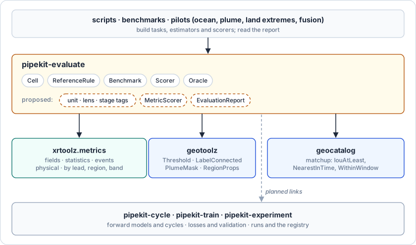
Figure 1:Ownership of evaluation. The dashed chips are the only new surface in pipekit-evaluate; the metrics stay where they are.
pipekit-evaluate owns the taxonomy tags, the scorer adapter, the evaluation report and the benchmark ladder. It depends on pipekit and only imports carrier libraries through extras.
The neighbours follow the stack rules. For this page, that means the metrics stay in xrtoolz (xarray carriers, with the decomposition wrappers) and geotoolz (GeoTensor detection blocks), neither of which imports pipekit-evaluate, and events become geocatalog rows (workstream E).
What the stack scores today¶
Table 2 is the scoping report’s matrix, filled with the names that ship at the pinned revisions, and Table 3 gives the decomposition wrappers beside it. Every cell which is not listed below is empty.
Table 2:The Lens × Unit matrix at the pinned revisions, one row per non-empty cell. All xrtoolz.metrics operators take (prediction, reference) datasets; “stub” is a reserved name that raises.
| Lens | Unit | Shipped |
|---|---|---|
| Point-wise | Field | RMSE, MSE, MAE, Bias, NRMSE, Correlation, R2Score, MaskedMetric, DieboldMariano |
| Point-wise | Statistic | BinnedResiduals2D, RegionScores |
| Probabilistic | Field | CRPS, SpreadSkillRatio, RankHistogram, EnsembleCoverage, ReliabilityCurve |
| Probabilistic | Statistic | EnergyDistance, Wasserstein1 |
| Spectral | Field | scores: PSDScore, psd_score, resolved_scale, WaveletPSDScore, FrequencyBandSkill, BandLimitedRMSE; tools in xrtoolz.transforms: power_spectrum, isotropic_power_spectrum, fit_spectral_slope, KESpectralFlux |
| Structural | Field | SSIM, GradientDifference, PhaseShiftError |
| Structural | Event | MaskIoU, CentroidDisplacement (pairs by label id); IntersectionOverUnion stub |
| Detection | Event | match_instances, InstanceF1AtIoU, AveragePrecisionMatched; stubs: ProbabilityOfDetection, FalseAlarmRatio, CriticalSuccessIndex, DurationError, IntensityBias |
| Physical-constraint | Field | GeostrophicBalanceError, GeostrophicImbalance, DivergenceError, DensityInversionFraction |
| Physical-constraint | Trajectory | PVConservationError (consumes trajectories nothing produces) |
| Physical-constraint | Budget | xrtoolz.budgets: BudgetResidual, HeatBudgetResidual, SaltBudgetResidual, VolumeBudgetResidual, KineticEnergyBudgetResidual |
Table 3:Decomposition wrappers at the pinned revisions.
| Wrapper | Shipped as | State |
|---|---|---|
| By lead time | xrtoolz.metrics.SkillByLeadTime(metric, lead_dim="lead_time") | shipped (Report 13) |
| By region | EvaluateByRegion(metric, *, regions); masks from xrtoolz.geo (REGIONS, RegionSpec, AddLandMask, eddy_regions) | shipped |
| By scale | FrequencyBandSkill(variable, dims, bands, metric=RMSE), evaluate_by_frequency_band; geo.BandpassWavelength as a pre-filter | shipped |
| By season or month | only viz.validation.seasonal_groupby, for plots | missing as a metric wrapper |
| By event | missing | |
| By member | inside each probabilistic metric’s ensemble_dim | missing as a wrapper |
We go through the scoping report’s gap analysis claim by claim, at the pinned revisions:
“xr_toolz.metrics has good point-wise coverage.” Partly: it covers far more than point-wise, although NSE and the index of agreement are missing.
“Spectral comparison is missing.” Wrong.
psd_score,PSDScore,WaveletPSDScore,resolved_scaleandFrequencyBandSkilllive inxrtoolz.metrics.spectral. What is missing is a comparison of two spectra which ignores phase (stage 1).“Structural (SSIM, FSS) is missing.” Partly: SSIM ships, whereas FSS, Hausdorff and perceptual losses do not.
“Detection is missing.” Partly: instance matching and an IoU-matched F1 ship, but event-level POD, FAR and CSI are reserved stubs.
“
xr_toolz.calchas gradients but no balance checks.” Wrong:xrtoolz.metrics.physicalhas geostrophic-balance, divergence, static-stability and PV-conservation errors.“No decomposition wrappers.” Wrong: lead time, region and frequency band ship; season, event and member do not.
“Trajectories and events are missing entirely.” Partly: trajectories are missing (
xrtoolz.metrics.lagrangianis an empty module marked “V3”), but event building blocks exist across geotoolz, xrtoolz and geocatalog.“
xr_toolz.budgetsexists but is not evaluation-shaped” and “no stage annotation”: hold.
The running example: one methane plume, three ways to get it wrong¶
The stages score the stack’s recurring object, a methane plume, against its truth. We use the shipped operators wherever they exist and mark hand-written code as user. The data are synthetic, so every score has a known right answer.
Stage 1 · The double penalty (Field × point-wise, structural, spectral)¶
TL;DR. Score a correctly shaped plume that is displaced, and a flat field that has no plume at all, and see which scores prefer which.
Problem. The truth is a Gaussian plume of peak 50 ppb and width cells on a periodic transect of cells, with the position along the transect (and a grid in 2-D). Prediction A, , is the same plume shifted by cells, and prediction B, , is the flat field at the truth’s mean. For a shift , the point-wise error of A is
where is the mean over the transect, and it overtakes the flat field’s RMSE once . So a score that sees the plume should prefer A.
1 2 3 4 5 6 7 8 9 10 11 12 13# Shapes: 1-D N = 40 cells; 2-D 64 × 64; A = plume shifted 6 cells, B = flat mean from xrtoolz.metrics import RMSE, SSIM, PhaseShiftError, psd_score RMSE("ch4", dims="x")(A, truth) # → 20.50 (B: 15.62) today PhaseShiftError("ch4", "x", periodic=True)(A, truth) # → shift_x = 6, residual_rmse = 0.0 (B: shift 0, residual 15.62) today psd_score(A, truth, psd_dims=["x"]) # mean over κ > 0: −1.105 (B: 0.0) today fss(A, truth, threshold=10, window=9) # → 0.625 (B: 0.0) user # relative spectrum difference Σ|P_A − P_x| / Σ P_x over κ > 0 spectrum_gap(A, truth) # → 0.000 (B: 1.000) user # 2-D 64 × 64: SSIM("ch4", ["y", "x"])(A2, truth2) # → 0.885 (B: 0.336) today RMSE("ch4", dims=["y", "x"])(A2, truth2) # → 4.671 (B: 4.096) today
Point-wise, structural and spectral scores on a displaced plume and a flat field, from a real run.
Table 4:Which scores prefer the displaced plume A over the flat field B.
| Score | Source | A | B | Prefers |
|---|---|---|---|---|
| RMSE (1-D) | xrtoolz.metrics.RMSE | 20.50 | 15.62 | B |
| RMSE (2-D) | xrtoolz.metrics.RMSE | 4.671 | 4.096 | B |
psd_score, mean over | xrtoolz.metrics.psd_score | −1.105 | 0.000 | B |
| SSIM (2-D) | xrtoolz.metrics.SSIM | 0.885 | 0.336 | A |
| Phase-shift residual | xrtoolz.metrics.PhaseShiftError | 0.0 (shift 6) | 15.62 | A |
| FSS, threshold 10, window 9 | user | 0.625 | 0.000 | A |
| Relative spectrum difference | user, over power_spectrum | 0.000 | 1.000 | A |
The double penalty is real, and the stack can already see past it (Table 4): SSIM and PhaseShiftError both prefer the plume, and PhaseShiftError even reports the 6-cell displacement. However, two lenses need code. FSS is not shipped (B1). In addition, the shipped spectral score is not the lens which the scoping report meant. psd_score compares the spectrum of the error with the spectrum of the truth, with the power spectral density at wavenumber , so it is phase-sensitive and suffers the double penalty too. A comparison of the two spectra, which ignores phase, prefers A perfectly, and it is a few lines over the shipped power_spectrum which belong beside psd_score (B1).
At the shift which the scoping report’s examples suggest, , RMSE still prefers the plume (15.44 against 15.62), because the flip needs for this width, as (1) predicts.
Stage 2 · Scale-blind aggregation (Statistic × spectral, by scale)¶
TL;DR. Blur a methane enhancement map and see how much the RMSE notices, then look at the spectrum and at the error scale by scale.
Problem. The truth is a field with an energy spectrum , normalised to unit standard deviation, where is the radial wavenumber in cycles per pixel. The prediction is the truth blurred by a Gaussian of width pixels. A blur multiplies the spectrum by , so the scale at which the error’s power reaches half the truth’s (the resolved scale) is known analytically, at 12.03 pixels.
1 2 3 4 5 6 7 8 9 10 11 12 13 14 15# Shapes: 128 × 128 pixels; κ in cycles per pixel from xrtoolz.metrics import FrequencyBandSkill, RMSE, SSIM, psd_score, resolved_scale from xrtoolz.transforms import fit_spectral_slope, isotropic_power_spectrum RMSE("z", dims=["y", "x"])(blur, truth) # → 0.098 of the truth's std today SSIM("z", ["y", "x"])(blur, truth) # → 0.885 today # slope of E(κ) over κ ∈ [0.05, 0.15] cycles / px fit_spectral_slope(isotropic_power_spectrum(truth.z, ["y", "x"]), k_min=0.05, k_max=0.15) # → −3.10 (blur: −9.39) today score = psd_score(blur.z, truth.z, psd_dims=["y", "x"], isotropic=True) resolved_scale(score, "freq_r", level=0.5) # frequency coordinate, 50 % level # → 11.98 px (analytic 12.03 px) today bands = {"large": (0, 0.05), "meso": (0.05, 0.125), "small": (0.125, 0.5)} FrequencyBandSkill("z", ["y", "x"], bands)(blur, truth) # → RMSE 0.053, 0.067, 0.049; divided by each band's truth std: 0.05, 0.60, 0.99
The blur scored point-wise, spectrally and by frequency band, from a real run.
The RMSE is under 10 % of the signal and SSIM is 0.885, yet the prediction has lost almost all of its variance below 8 pixels, and its spectral slope is −9.4 where the truth’s is −3.1. The shipped tools see this. resolved_scale recovers the analytic 12-pixel scale to 0.4 %, and FrequencyBandSkill shows the small-scale error at 99 % of that band’s signal. So the scoping report’s spectral lens and “by scale” wrapper exist, and the one missing piece is a score that compares the two slopes directly (B1).
Stage 3 · Did it find the plumes? (Event × detection)¶
TL;DR. Detect plumes in a predicted and a reference map, match them, and count hits, misses and false alarms.
Problem. The reference map has two plumes. The prediction has the first one shifted by 3 pixels, misses the second, and adds one false alarm. With hits, false alarms and misses (all counts), the detection scores are (2), (3) and (4),
where each score is a scalar in .
1 2 3 4 5 6 7 8 9 10 11 12 13# Shapes: two label images; masks (n_objects, H, W) from xrtoolz.metrics import instance_f1_at_iou, mask_iou_matrix, match_instances labels_ref, labels_pred = label(ref > 0.3), label(pred > 0.3) # scipy user mask_iou_matrix(pred_masks, ref_masks) # → [[0.438, 0], [0, 0]] today match_instances(pred_masks, ref_masks, iou_threshold=0.3) # → tp = 1, fp = 1, fn = 1 today instance_f1_at_iou(pred_masks, ref_masks, iou_threshold=0.3) # → F1 = 0.5 today # POD = N_hit / (N_hit + N_miss) = 0.5; FAR = N_false / (N_hit + N_false) = 0.5 user # CSI = N_hit / (N_hit + N_false + N_miss) = 0.333 user CriticalSuccessIndex() # → NotImplementedError: … a name reservation; implementation lands with V5 centroid_displacement(pred_objects, ref_objects) # → pairs object 2 with object 2: 30.6 px between unrelated plumes
Event detection and matching with what ships, from a real run.
Matching works, since match_instances counts the hit, the miss and the false alarm correctly, and the scores in (2) to (4) follow from its counts in one line each. However, they are not shipped, although their names are reserved in xrtoolz.metrics.object (B2). CentroidDisplacement pairs objects by label id rather than by matching, so it compares unrelated plumes when the labels are not aligned, and it should take the pairing of match_instances instead (B2). Detection itself is assembled from geotoolz (segment.Threshold, measure.LabelConnectedComponents, plume.PlumeMask) and xrtoolz (remove_small_objects_2d). What does not exist is an event as an object with an id, a time span and attributes (E).
Stage 4 · The benchmark ladder (pipekit-evaluate)¶
TL;DR. Score three estimators of the same linear-Gaussian retrieval with the ladder pipekit-evaluate ships: an exact oracle, a prior-only baseline and an over-confident shortcut.
Problem. The state , with cells, is drawn from with a squared-exponential covariance of length 3 cells. Every fourth cell is observed, so with , , the selection matrix and with . The oracle is the exact posterior mean and its covariance . The ladder places each estimator in a cell (level, rung, complexity) and scores it against the reference which its rung calls for, namely the known truth for model-based inference and the oracle’s posterior for an amortized predictor.
1 2 3 4 5 6 7 8 9 10 11 12 13# Shapes: x (40,); y (10,) import pipekit_evaluate as pev report = pev.Benchmark( task=LGTask(), # 40 cells, every 4th user estimators=[ExactOI(), ZeroPrior(), WrongRidge()], # user scorers=[RMSE(), GaussCoverage()], # pev.Scorer protocol user level="L4", ).run() # today # L4/r2/c1 model_based_inference ref=known_theta rmse 0.406 cov90 0.825 # L4/r2/c0 model_based_inference ref=known_theta rmse 0.569 cov90 0.975 # L4/r5/c0 amortized_predictor ref=oracle_posterior rmse 0.597 report.to_dict() # {cell label: {metric: value}}; drops reference and notes
A benchmark on the shipped ladder, from a real run. The task, estimators and scorers are user code.
The ladder runs and resolves references as its design says. The exact oracle beats the prior-only baseline against the truth, and the over-confident shortcut is scored against the oracle’s posterior and not the truth. However, it took about 80 lines of glue, and the run exposed six frictions, which are all in Section ??:
No carriers ship. The Gaussian prior, the estimate, the observation operator and a no-op forward model for a static problem are all user code, and
Benchmarknever calls the task’sprior(),simulator()orobservation_operator().One reference per cell. The amortized rung cannot be scored against both the oracle and the truth in one run.
Estimatehas no covariance. So a coverage scorer must read a covariance by duck typing, or sample.The complexity axis scores the oracle against a worse baseline (RMSE 0.735 of the exact posterior against the prior), and its note for a step-0 cell says “generative rung”, which a step-0 cell is not.
The docstring and the code disagree on which estimator becomes the oracle (
run.py:77says the lowest complexity; the code takes the highest).to_dictdrops the reference, the note and the axis, and nothing hashes, tables or logs the report.
Report 17 runs the same ladder on rungs 2 to 5 of one retrieval, including the emulator rungs 3 and 4 which this stage leaves empty.
Stage 5 · What cannot be scored yet: trajectories¶
TL;DR. The Lagrangian unit has no producer in the stack.
Problem. For a velocity field at location and time , a particle path solves . Dispersion is the mean squared separation of initially close pairs, and the finite-time Lyapunov exponent is the growth rate of that separation. So scoring a forecast’s transport skill needs particles which are advected through both the forecast and the reference velocity.
Nothing in the pinned stack advects a particle. xrtoolz.metrics.lagrangian is an empty module reserved for “V3”, PVConservationError takes trajectories as input but nothing produces them, and viz.validation.EulerianLagrangianPanel plots them. Workstream D adds the producer in xrtoolz and the scores beside the reserved module. There is no run here.
The scoping report’s names, checked¶
Table 5 checks the stack names the scoping report’s examples use.
Table 5:The stack names the scoping report’s examples use, at the pinned revisions.
| Name in the report | At the pinned revisions |
|---|---|
pe.Pipeline([...]).run(predictions, reference), run_on_matched | do not exist; pipekit_evaluate.Benchmark(task, estimators, scorers, ...).run() |
pe.metrics.pointwise.RMSE(), pe.metrics.probabilistic.CRPS(ensemble_dim=...) | in xrtoolz: xrtoolz.metrics.RMSE(variable, dims), CRPS(variable, *, ensemble_dim, dims) |
pe.ByLeadTime, pe.ByRegion(regions=..., metric=...) | in xrtoolz: SkillByLeadTime(metric, lead_dim), EvaluateByRegion(metric, *, regions) |
pe.metrics.spectral.PSDCompare(expected_slope=-3.0, tolerance=0.5) | does not exist; fit_spectral_slope and psd_score do (stage 2) |
pe.metrics.physical.MassClosure(tolerance=0.01) | does not exist; xrtoolz.budgets.BudgetResidual and the per-quantity residuals do |
pe.ByEvent, pe.events.MarineHeatwaveDetector, pe.metrics.detection.CSI() | do not exist; CriticalSuccessIndex is a reserved stub in xrtoolz.metrics.object |
pe.adapters.train.MetricAsLoss, EvaluationCallback, pe.MetricObserver | do not exist |
registry.attach_evaluation(model_hash=..., report=...) | does not exist (Report 12) |
sc.DuckDBStateCatalog, state_cat.queries.forecast_chain, latest_analysis | not built; Report 13 proposes geocatalog.states.forecast_chain and latest_analysis |
gc.queries.matchup(primary, secondary, time_tolerance, space_tolerance_km) | geocatalog.matchup.matchup(primary, secondary, *, spatial, temporal, ...) with strategies such as NearestInTime(dt) |
pipekit_evaluate.presets.weatherbench(), oceanbench() | do not exist; the four pilots are design docs |
pe as the import alias | these reports use pev for pipekit-evaluate and px for pipekit-experiment |
Current-state audit¶
Of the fourteen pieces we checked, eight ship and work, three ship with defects or gaps, and three are missing (Table 6), and Figure 2 counts the page’s calls by marker. The audit read the pinned revisions on 13 October 2026.
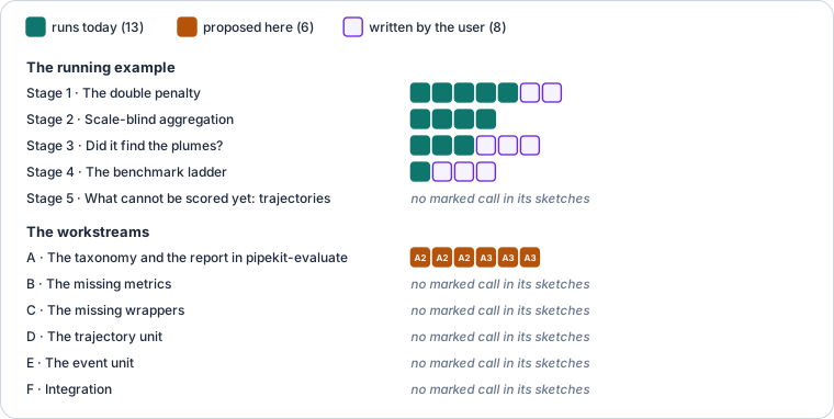
Figure 2:What this page’s sketches call: of 27 stack calls, 13 run today, 6 are proposed by this report’s workstreams and 8 are code the reader writes (how to read it).
Table 6:Evaluation in the stack, piece by piece.
| Symbols | Defined in | Used by | Verdict |
|---|---|---|---|
Cell, RUNG_NAMES, LEVEL_NAMES | pipekit_evaluate/benchmark/cube.py | the ladder | Healthy. Levels L0 to L4, six rungs |
ReferenceRule, ReferenceSource, Axis | benchmark/reference.py | Benchmark | Split ownership. One source per cell; PREVIOUS_RUNG unused |
Prior, Estimate, Task, Estimator, Oracle, Scorer | benchmark/protocols.py | stage 4 | Split ownership. No carriers ship; Oracle is “not yet consumed”; Estimate has no covariance |
Benchmark, BenchmarkReport, CellResult | benchmark/run.py | stage 4 | Split ownership. to_dict only; docstring and code disagree on the oracle |
| Unit × Lens × Stage taxonomy | pipekit_evaluate/__init__.py:3, README | Missing. “still planned” | |
| point-wise and probabilistic field metrics | xrtoolz.metrics | Report 13 stage 4 | Healthy. NumPy, xskillscore |
| spectral scores and tools | xrtoolz.metrics.spectral, xrtoolz.transforms | stage 2 | Healthy. resolved_scale within 0.4 % of the analytic value |
| structural field metrics | xrtoolz.metrics (SSIM, PhaseShiftError) | stage 1 | Healthy. FSS missing |
| instance matching | xrtoolz.metrics (match_instances, InstanceF1AtIoU) | stage 3 | Healthy. |
| event detection scores | xrtoolz.metrics.object | Missing. Reserved stubs | |
| physical-constraint and budget residuals | xrtoolz.metrics.physical, xrtoolz.budgets | Healthy. Not run here; residuals, not prediction-against-reference scores | |
| decomposition wrappers | xrtoolz.metrics (SkillByLeadTime, EvaluateByRegion, FrequencyBandSkill) | stage 2, Report 13 | Healthy. Season, event, member missing |
| trajectories | xrtoolz.metrics.lagrangian | Missing. Empty module | |
| the capability index | geostack scripts/capabilities.py | every scoping report | Healthy as code, misleading in scope: four xrtoolz names |
Smaller findings:
No metric is differentiable or stage-tagged. xrtoolz’s kernels are NumPy (
_pixel_kernels.py: “Backend: numpy. JAX / CuPy variants are out of scope”), none of them carries a flag, and the differentiable losses live inpipekit_train.loss.pot_exceedancesreturns exceedances, not events. They have no ids or durations, so marine-heatwave-style events need a detector (E1).The pilots name libraries which this audit did not check (somax, vardax, plumax, xtremax, filterax, gaussx). Their scorer lists (SBC, coverage, twCRPS, C2ST, Okubo–Weiss detection, triple collocation) are the best catalogue of what the ladder will need.
pipekit-evaluate’s extras are
cycle,xskillandproper, and thexskillandproperextras have no code behind them yet.
Workstream A · The taxonomy and the report in pipekit-evaluate¶
Decision. pipekit-evaluate’s Scorer carries the taxonomy as data, any metric operator becomes a scorer through one adapter, and the ladder’s report becomes the scoping report’s EvaluationReport (Table 7).
Table 7:Workstream A’s moves.
| Symbol | Destination | Reason |
|---|---|---|
unit, lens, stages, differentiable attributes | Scorer protocol (optional, with defaults) | the scoping report’s Metric protocol, as metadata on the seam that already exists |
MetricScorer(metric, *, unit, lens, stages, reference="truth") | pipekit_evaluate.scorers | wraps any (prediction, reference) → Dataset operator (every xrtoolz.metrics operator) as a Scorer |
EvaluationReport with ReportEntry(metric, lens_path, value, unit, stage) | pipekit_evaluate.report | BenchmarkReport plus model_ref, dataset_ref, config, timestamp; content_hash, to_pandas, filter, diff |
several references per cell; covariance on Estimate; complexity-axis wording; oracle docstring | benchmark/ | stage 4’s frictions |
1 2 3 4 5 6 7 8 9 10 11 12# Shapes: as stage 1; xm is xrtoolz.metrics scorers = [ pev.MetricScorer(xm.RMSE("ch4", dims="x"), unit="field", lens="pointwise", stages={"validation", "final"}), # proposed (A2) pev.MetricScorer(xm.SSIM("ch4", ["y", "x"]), unit="field", lens="structural", stages={"final"}), # proposed (A2) pev.MetricScorer(xm.FSS("ch4", threshold=10, window=9), unit="field", lens="structural", stages={"final"}), # proposed (A2, B1) ] report = pev.evaluate(prediction, truth, scorers, model_ref=h) # proposed (A3) report.filter(lens="structural").to_pandas() # proposed (A3) report.diff(last_week) # per-entry changes proposed (A3)
Stage 1’s scores as tagged scorers in one report, after workstream A.
Workstream B · The missing metrics¶
Decision. Each missing metric goes into the xrtoolz module which already holds its lens, under the name it reserves where one is reserved (Table 8).
Table 8:Workstream B’s moves.
| Symbol | Destination | Reason |
|---|---|---|
FSS(variable, *, threshold, window) | xrtoolz.metrics (structural) | stage 1; the scoping report’s main structural score |
SpectrumDistance, SpectralSlopeError(k_min, k_max) | xrtoolz.metrics.spectral | stage 1 and 2: compares two spectra, ignoring phase |
ProbabilityOfDetection, FalseAlarmRatio, CriticalSuccessIndex, ContingencyTable | xrtoolz.metrics.object (the V5 stubs) | stage 3; built on match_instances |
CentroidDisplacement on matched pairs | xrtoolz.metrics.object | stage 3: pairs by label id today |
NSE, IndexOfAgreement, BrierScore, EnergyScore | xrtoolz.metrics | missing point-wise and probabilistic cells |
HausdorffDistance, StructureFunction | xrtoolz.metrics | missing structural and spectral cells |
Workstream C · The missing wrappers¶
Decision. Three more wrappers join SkillByLeadTime, EvaluateByRegion and FrequencyBandSkill, and they have the same shape: a metric goes in, and a dataset with one more dimension comes out (Table 9).
Table 9:Workstream C’s moves.
| Symbol | Destination | Reason |
|---|---|---|
EvaluateByGroup(metric, *, by="time.season") | xrtoolz.metrics | by season or month; only a plotting groupby exists |
EvaluateByEvent(metric, *, events) | xrtoolz.metrics | restricts a metric to event masks or matched pairs |
EvaluateByMember(metric, *, ensemble_dim) | xrtoolz.metrics | per-member scores for point-wise metrics (Report 13’s C2 broadcasting is the same need) |
Workstream D · The trajectory unit¶
Decision. Particle advection is a transform over velocity fields, so it lives in xrtoolz, and trajectory scores live in the module which xrtoolz reserves for them (Table 10).
Table 10:Workstream D’s moves.
| Symbol | Destination | Reason |
|---|---|---|
AdvectParticles, PairDispersion, FTLE | xrtoolz.lagrangian (new), with an optional diffrax backend | nothing advects particles today; the scoping report’s §3.1 |
TrajectoryRMSE, SeparationDistance, DispersionCRPS | xrtoolz.metrics.lagrangian (reserved “V3”) | the trajectory column of the matrix; PVConservationError gains a producer |
Workstream E · The event unit¶
Decision. Events are detected with the stack’s segmentation tools and stored as catalog rows with an event profile, and not in a third catalog type (Table 11).
Table 11:Workstream E’s moves.
| Symbol | Destination | Reason |
|---|---|---|
ThresholdEventDetector, MarineHeatwaveDetector (percentile, minimum duration) | xrtoolz.events (new) over geotoolz.segment and xrtoolz.geo.pot_threshold | stage 3’s labels are scipy calls; pot_exceedances has no ids or durations |
event rows: event_id, kind, start, end, footprint, attributes, source_uri | a geocatalog event profile (geocatalog.events), like Report 13’s state profile | the scoping report’s EventCatalog, without a parallel index; matching through geocatalog.matchup (IouAtLeast, NearestInTime) |
Workstream F · Integration¶
Decision. Evaluation connects to training, cycles and the registry through the seams which those packages already have, or which their own reports propose (Table 12).
Table 12:Workstream F’s moves.
| Symbol | Destination | Reason |
|---|---|---|
a scorer with differentiable=True as a pipekit-train Loss | pipekit-evaluate adapter over pipekit_train.loss | the scoping report’s MetricAsLoss; refuses non-differentiable scorers, which today means every xrtoolz metric |
| per-step scoring in cycles | the on_step(k, carriers, state) hook of Report 13’s open question 3 | the scoping report’s MetricObserver; a step inside a Sequential is rejected by cycles today (Report 10, workstream A) |
| a report linked to its model | registry metadata (Report 12, workstream C) | the scoping report’s attach_evaluation |
presets.plume(), presets.ocean(), presets.land_extremes(), presets.fusion() | pipekit-evaluate | the four pilots’ scorer lists, in place of weatherbench() and oceanbench() |
Testing gates¶
Each workstream only merges when its gates pass, and the existing gates are checks which the code passes today (Table 13).
Table 13:Gates for the proposals and for what ships.
| Gate | Workstream | Passes when |
|---|---|---|
| A1 Tags | A1 | every scorer in stage 4 and A2’s example reports its unit, lens and stages; an untagged scorer defaults to unit “field”, lens “pointwise” |
| A2 Adapter parity | A2 | MetricScorer(xm.RMSE(...)) returns stage 1’s 20.50 and 15.62 to 1e-12 |
| A3 Report | A3 | content_hash is equal for two runs of stage 1 and differs when one value changes; filter(lens="structural") returns exactly the structural entries; diff against itself is empty |
| A4 Ladder | A4 | stage 4’s rung 5 gets both oracle and truth scores in one run, and to_dict keeps the reference source |
| B1 FSS and spectra | B1 | FSS equals stage 1’s 0.625 (1-D, window 9) and 0.566 (2-D); SpectrumDistance is 0 for any circular shift and 1.0 for the flat field |
| B2 Detection | B2 | on stage 3, POD = 0.5, FAR = 0.5, CSI = 1/3 exactly, and CentroidDisplacement reports 3 px for the matched pair only |
| B3 Scores | B3 | NSE of a perfect prediction is 1 and of the reference mean is 0; Brier of a perfect probability forecast is 0 |
| B4 Shape scores | B4 | Hausdorff distance of a plume and its 6-cell shift is 6 cells |
| C1 to C3 Wrappers | C | each wrapper’s per-group values equal the metric applied by hand to each group, to 1e-12 |
| D1 Advection | D1 | particles in a uniform flow move to 1e-6; pair dispersion in a linear strain of rate grows as to 1 % |
| D2 Trajectory scores | D2 | TrajectoryRMSE of identical paths is 0 |
| E1 Detector | E1 | a synthetic heatwave of known start, end and peak is detected with those values |
| E2 Event rows | E2 | stage 3’s events round-trip through GeoParquet, and matchup(IouAtLeast(0.3)) reproduces match_instances’ pairing |
| F1 to F4 Integration | F | a differentiable scorer trains Report 11’s emulator to the same weights as MSE to 1e-6; a preset runs on its pilot’s toy task |
| S1 Resolved scale (existing) | — | stage 2’s resolved_scale within 1 % of the analytic 12.03 px. Passes today: 11.98 |
| S2 Phase shift (existing) | — | stage 1’s PhaseShiftError returns the true shift with zero residual. Passes today |
| S3 Matching (existing) | — | stage 3’s match_instances returns tp = fp = fn = 1. Passes today |
Sequencing and risks¶
The taxonomy and report come first, because they need no new metrics and they make every later metric land in a structured place. The metrics fill the matrix next, then the two new units, and then the integrations (Figure 3).
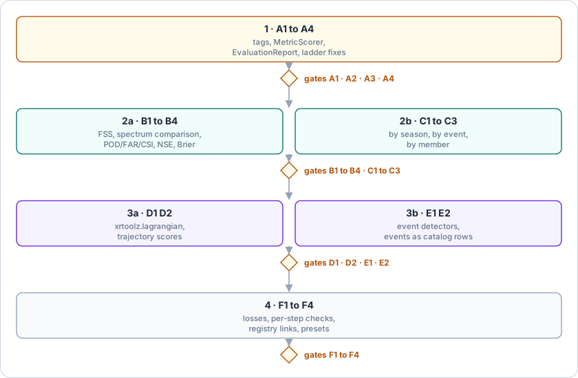
Figure 3:The taxonomy and report first, then the metrics, then the new units, then the integrations.
Two homes for metrics. Tags in pipekit-evaluate and code in xrtoolz could drift. Fallback: the tags live on the
MetricScorerwrapper and not on xrtoolz operators, so xrtoolz never depends on the taxonomy.Differentiable lenses do not exist yet. Every xrtoolz metric is NumPy, so the Stage axis’s “training” column is empty except for pipekit-train’s losses. Fallback: F1 only accepts
pipekit_train.lossobjects and JAX scorers until xrtoolz grows JAX kernels.Spectral scores are sensitive to windows and detrending. Stages 1 and 2 passed
window=Noneanddetrend=None, and the defaults change the numbers. Fallback: every spectral scorer records its spectral options in its report entry.Event detection is domain-specific. Plumes, heatwaves and eddies need different detectors. Fallback: we ship two reference detectors (threshold plus connected components, and the heatwave rule) and leave the rest to domain libraries.
Lagrangian evaluation is expensive. Advecting many particles over long windows is for final evaluation only. Fallback: we tag trajectory scorers
stages={"final"}and provide subsampled variants.
Open questions¶
Does the taxonomy belong on the metric or on the scorer? This page puts it on the scorer (A1). However, if xrtoolz operators carried it too, a catalogue of the whole matrix could be generated from the code.
One report type or two?
BenchmarkReport(rung by rung) and the scoping report’sEvaluationReport(lens by lens) could be one class with two views, or two classes.Should events live in geocatalog? The event profile follows Report 13’s decision for states. Events also carry lineage to the field they were detected in, so is a
source_uricolumn enough?Where do differentiable metrics come from? JAX versions of xrtoolz kernels, a pipekit-jax metric set, or pipekit-train losses only?
What should the capability index cover? Indexing every xrtoolz subpackage adds hundreds of names. Should it cover all of them, or only the public namespaces (
metrics,transforms,geo,ocn,budgets)?
Upcoming work¶
Table 14 lists the follow-ups.
Table 14:Follow-ups from checking the scoping report against the code.
| Follow-up | Where | Why |
|---|---|---|
| Index xrtoolz’s and geocatalog’s subpackages | geostack scripts/capabilities.py (UPSTREAM), then make capabilities | the index lists four xrtoolz names, so scoping from it misses most of this matrix |
| Fix the oracle docstring and the step-0 note | pipekit-evaluate benchmark/run.py:77, :205 | stage 4 |
Give BenchmarkReport.to_dict the reference, note and axis | pipekit-evaluate | stage 4 |
Document psd_score as an error-spectrum score | xrtoolz.metrics.spectral | stage 1: it is phase-sensitive, unlike a spectrum comparison |
Remove or implement the xskill and proper extras | pipekit-evaluate pyproject.toml | no code uses them |
References¶
Sources¶
The scoping report, “Report 14 —
pipekit-evaluate: multidimensional evaluation as first-class infrastructure” (supplied by the author).pipekit-evaluate 0.0.2 in
references/geostack/pipekit/packages/pipekit-evaluate: its source, tests, README, CHANGELOG,benchmark_ladder.mdand the four pilot designs.xrtoolz 0.0.5 (
xrtoolz.metrics,.transforms,.geo,.budgets), geotoolz and geocatalog at the pinned revisions.The running example’s scripts and outputs, described in Section ??.