diagnostix: diagnostics of geophysical fields for JAX
diagnostix computes what a geophysical field says, physically and statistically: kinematics (vorticity, strain, Okubo–Weiss, geostrophy, potential vorticity), column quantities (N², mixed-layer depth, boundary-layer height, column integrals), budgets, climatologies and anomalies, spectra, area-weighted EOFs and skill scores. It sits at GeoNumerics tier 2, on gridax’s differences, and holds the maths that xrops wraps for xarray. It absorbs what was planned as skillax. Status: proposed, at design-sketch depth.
At a glance
| Layer, tier | GeoNumerics, tier 2 |
| Imports | gridax, geophysix, functax; JAX, NumPy, SciPy |
| Imported by | xrops; sesmax-ocean (planned) |
| Takes over | the maths of xrops ocn, atm (vertical and wind), budgets, anomaly, the spectra and decompositions in transforms and wavelets, and the scores in metrics; somax’s eval/metrics.py |
| Does not own | the DataArray API (xrops); differences and metrics (gridax); bases and generic signal processing (functax); benchmark contracts and leaderboards (pipekit-evaluate); extremes modelling (xtremax) |
| Status | proposed; no repository yet |
| Tracked in | the layer map; the companion gridax and functax designs |
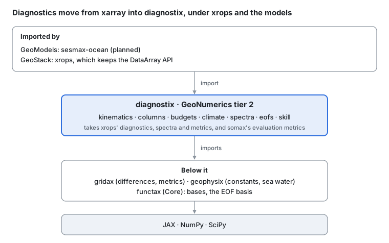
Where diagnostix sits · geonumerics tier 2.
diagnostix sits one tier above gridax, whose differences and metrics every diagnostic is built from. This page is the design; core types, algorithms and the code survey are in diagnostix: design details.
The problem
A plume’s emission rate is checked with diagnostics before anyone trusts it, and every one of them lives in xrops, on xarray, in NumPy and SciPy:
| Step | The diagnostic | Where it is coded today |
|---|---|---|
| How deep the plume mixes | boundary-layer height from the bulk Richardson number | xrops pbl_height_bulk_richardson |
| The enhancement over background | a climatology and the anomaly from it | xrops calculate_climatology, calculate_anomaly and their smoothed forms |
| The rate by mass balance | the flux through the faces of a box around the source | xrops boundary_flux (which sums over every face of the field, not a chosen box), control_volume_integral, budget_residual |
| Which scales a reconstruction resolves | power spectra and the PSD score | xrops power_spectrum, isotropic_power_spectrum, psd_score, resolved_scale |
| How good the transport model is | RMSE, bias, correlation, spread–skill | xrops metrics (rmse, bias, correlation, spread_skill_ratio, rank_histogram) |
| The ocean side, for sesmax | vorticity, strain, Okubo–Weiss, geostrophy, kinetic energy | xrops ocn/kinematics.py; somax eval/metrics.py; finitevolX operators/diagnostics.py on its C-grid |
Because they sit on xarray, none of them traces under JAX or differentiates, so a model that wants a diagnostic inside its loop or as a loss writes it again: kinetic energy, enstrophy and geostrophic imbalance each exist in xrops, in somax and in finitevolX. And xrops’ diagnostics run on geoops’ difference kernels, so the xarray toolkit depends on the GeoArray toolkit for maths that belongs to neither.
What a field says
A diagnostic is a function of one or more fields on a grid that returns a smaller or more telling field: a derivative combination, an integral, a residual, a spectrum, a decomposition or a score. Each is built from gridax’s differences and metrics and geophysix’s constants.
Kinematics. With u, v the horizontal velocity and f the Coriolis parameter, vorticity and the two strains are
The Okubo–Weiss parameter Okubo, 1970Weiss, 1991 W = σₙ² + σₛ² − ζ² separates strain-dominated from rotation-dominated flow, and the geostrophic velocity from sea-surface height η is u_g = −(g / f) ∂ᵧη, v_g = (g / f) ∂ₓη.
Columns. The buoyancy frequency is N² = −(g / ρ₀) ∂ρ/∂z with ρ from geophysix’s equation of state. The boundary-layer height is the lowest z where the bulk Richardson number reaches a critical value Ri_c, with θ_v the virtual potential temperature:
Budgets. For a quantity q carried by the velocity u, with source S, over a control volume V with surface ∂V and outward normal n,
and the residual of that balance is the diagnostic. For a plume in steady state, the flux through the faces of a box around the source is the emission rate, Q = ∮ Ω’ (u · n) dl, with Ω’ the column enhancement.
Climate. With q̄(d) the climatology at calendar day d (on a leap-year calendar, so each date keeps one slot in every year), the anomaly is q’(t) = q(t) − q̄(d(t)); trends, detrending and temporal filters act on q’.
Spectra. With q̂(k) the Fourier transform of q, the power spectrum is P(k) = |q̂(k)|², the isotropic spectrum averages it over rings of |k|, and the spectral flux Π(k) sums the nonlinear transfer below k. Cross, coherence and rotary spectra and wavelets follow the same pattern.
EOFs. With X the anomaly matrix (time × space) and W the diagonal of cell areas from gridax, the area-weighted EOFs come from the SVD of the weighted anomalies:
The EOFs are W^(−1/2) U, the principal components VΣ, and the i-th explains a fraction σᵢ² / ∑ⱼ σⱼ² of the variance.
Skill. With ŷ a prediction and y the truth over valid cells with weights w, RMSE = (∑ w (ŷ − y)² / ∑ w)^½, the bias, the correlation, and for ensembles the spread–skill ratio and the rank histogram.
Modules and boundaries
Seven modules. Every function takes arrays and a gridax grid and returns arrays; xrops keeps the names, attributes and units.
| Module | Owns | Comes from |
|---|---|---|
diagnostix.kinematics | vorticity, divergence, strains, Okubo–Weiss, geostrophic and ageostrophic velocity, kinetic energy and enstrophy, frontogenesis, potential vorticity | xrops ocn/kinematics.py; somax eval/metrics.py |
diagnostix.columns | N², lapse rate, mixed-layer depth, boundary-layer height, column integrals | xrops ocn/kinematics.py (N², mixed layer), atm/_src/vertical.py |
diagnostix.budgets | control-volume integrals, boundary fluxes, budget residuals for volume, heat, salt, kinetic energy and tracer mass | xrops budgets/ |
diagnostix.climate | climatologies, anomalies, trends, detrending, temporal filters | xrops anomaly/ |
diagnostix.spectra | power, isotropic, cross, coherence and rotary spectra, spectral fluxes, slopes, wavelets | xrops transforms/_src/fourier.py, wavelet.py, wavelets/ |
diagnostix.eofs | area weighting and the analysis of EOFs: explained variance, principal components, truncation | xrops transforms/_src/decompose.py (eof, pca), which are unweighted scikit-learn PCA; the area weighting is new |
diagnostix.skill | pixel, spectral, probabilistic and physical scores: RMSE, bias, correlation, PSD score, resolved scale, spread–skill, rank histogram, geostrophic and PV residuals | xrops metrics/; somax eval/metrics.py |
What diagnostix owns, and what it hands off
The test for every name: does it take a field on a grid and say something about it, physically or statistically? Then diagnostix owns it.
| Neighbour | diagnostix owns | The neighbour owns | The line |
|---|---|---|---|
| xrops | the maths | the DataArray API: names, attributes, units, dask chunking | xrops calls diagnostix kernels |
| gridax | the diagnostics | differences, metrics, vertical coordinates on analysis grids | diagnostix composes gridax’s differences |
| functax | the area weighting and the analysis of EOFs | bases, including an EOF basis from data; generic signal processing | the basis is functax’s, what it says about the climate is diagnostix’s |
| finitevolX | diagnostics on an A-grid | operators and conserved quantities on a model’s C-grid | in a model’s own staggering, finitevolX (decision 4) |
| pipekit-evaluate | the scores | benchmark contracts, evaluation protocols, leaderboards | a score is a function here; a benchmark that runs it is pipekit’s |
| xtremax | anomalies and climatologies | extremes modelling: GEV, GPD, return levels | xtremax fits extremes to what diagnostix extracts |
What moves in
| From | What | Its users then import |
|---|---|---|
| xrops | the maths of ocn, atm (vertical and wind), budgets, anomaly, the spectra and decompositions in transforms and wavelets, and metrics | diagnostix underneath; xrops keeps every DataArray function and Operator, and metrics/leaderboard.py goes to pipekit-evaluate |
| somax | eval/metrics.py: kinetic energy, enstrophy, RMS divergence, geostrophic imbalance, QG balance residual | diagnostix.kinematics, diagnostix.skill; sesmax-core inherits nothing to move |
| the skillax plan | skill scores | diagnostix.skill (decision 2) |
In use
Checking a plume’s emission rate: how deep it mixes, its enhancement over background, its rate by mass balance, and how well the transport model reproduces it. Every diagnostix name is proposed.
# Shapes: Z levels; T times; Ny × Nx lon/lat cells

import diagnostix as dgx
import gridax as gdx

# proposed (gridax)
grid = gdx.grids.SphericalGrid.from_axes(lon_centres, lat_centres, stagger="A")

# --- how deep the plume mixes ---
# proposed (diagnostix)
# lowest z where Ri_b(z) = (g / θ_v0) (θ_v(z) − θ_v0) z / (u² + v²) reaches Ri_c
mixing_height = dgx.columns.boundary_layer_height(  # (Z, Ny, Nx) → (Ny, Nx)
    virtual_potential_temperature, eastward_wind, northward_wind, heights
)

# --- enhancement over background ---
# proposed (diagnostix)
# Ω' = Ω − Ω̄(d(t))
enhancement = dgx.climate.anomaly(column, climatology, day_of_year)  # → (T, Ny, Nx)

# --- the rate by mass balance ---
# proposed (diagnostix)
# Q = ∮ Ω' (u · n) dl over the faces of the box
rate = dgx.budgets.boundary_flux(  # (T, Ny, Nx) → (T,)
    grid, enhancement, eastward_wind_pbl, northward_wind_pbl, box=source_box
)

# --- skill of the transport model ---
# proposed (gridax)
cell_area = gdx.metrics.cell_area(grid)  # → (Ny, Nx)
# proposed (diagnostix)
# RMSE = (∑ w (ŷ − y)² / ∑ w)^½, with w the cell areas
error = dgx.skill.rmse(simulated, enhancement, weights=cell_area)  # → (T,)
Each call is a pure JAX function, so the same rmse and boundary_flux can sit inside a training loss for an emulator of the transport model, where today they cannot.
Integration across the stack
Two libraries would import diagnostix, and one model’s metrics retire into it.
| Consumer | Uses today | With diagnostix |
|---|---|---|
| xrops | every diagnostic written on xarray in NumPy and SciPy, its differences through geoops | the same DataArray functions and Operators, each a thin wrapper over a diagnostix kernel; differences through gridax, so xrops’ calculus no longer needs geoops |
| sesmax-ocean (planned) | — | kinematics, spectra and skill as in-loop diagnostics and losses |
| somax | eval/metrics.py | retires with somax; sesmax-ocean imports diagnostix instead |
For an xrops user nothing changes; inside xrops the kernel moves:
# Today: xrops computes ζ on xarray with geoops' difference kernels
# today (xrops)
from xrops.ocn import relative_vorticity

# After: the same function, a wrapper over the JAX kernel
# proposed (diagnostix)
from diagnostix.kinematics import vorticity
Decisions and open questions
Four decided, two leaning, one open. Each entry gives the position first, then the trade-off.
1. Layer: GeoNumerics tier 2
Decided (5 Nov 2026, on the layer map). diagnostix imports gridax (tier 1), geophysix (tier 0) and functax (Core). xrops and sesmax-ocean sit above it.
2. One library for physical and statistical diagnostics
Decided (5 Nov 2026). The skill scores planned for a separate skillax live here. A PSD score and a resolved scale need the same spectra as an energy-flux diagnostic, and a geostrophic-imbalance score needs the same kinematics; two libraries would import each other.
3. The DataArray API stays in xrops
Decided (5 Nov 2026, on the layer map). diagnostix takes arrays and a gridax grid. Names, attributes, units, CF conventions and dask chunking are xrops’, which wraps each kernel.
4. Diagnostics on a model’s own grid
Open. finitevolX’s operators/diagnostics.py computes kinetic energy, strain, Okubo–Weiss, enstrophy, QG potential vorticity and available potential energy in its C-grid staggering, as functions, as masked classes and as pipekit Operators, as a model steps. Leaning: those stay in finitevolX, because they are operators on the model’s state; diagnostix’s versions work on A-grid fields as they arrive from a model’s output or a product. somax’s evaluation metrics, which work on outputs, move here. Either way diagnostix never imports finitevolX: finitevolX is GeoNumerics tier 3 and diagnostix tier 2, and an optional import still counts as an edge. If both come to need one kernel, it moves down into diagnostix (or gridax) and finitevolX imports it.
5. JAX kernels, SciPy where it must be
Leaning. Everything a loss might use (kinematics, columns, budgets, spectra, skill) is a traceable JAX function. The few routines that rest on host-only libraries today (PyWavelets for wavelets, xrft for spectra, scikit-learn for EOFs) may stay on the host behind the same names, marked as such, until a JAX version is worth writing.
6. EOFs: the basis in functax, the analysis here
Decided (5 Nov 2026, on the layer map). functax builds a basis from data with weights as an argument; diagnostix supplies the area weights from gridax, the truncation and the reading of the modes.
7. Scores here, benchmarks in pipekit-evaluate
Leaning. A score is a function of a prediction and a truth; a benchmark that fixes the data, the splits and the leaderboard is pipekit-evaluate’s. xrops’ metrics/leaderboard.py moves there, not here.
Roadmap
Six waves, each a GitHub issue epic in the diagnostix repository once it exists.
| Wave | Delivers | Ends | Needs |
|---|---|---|---|
| 0. Scaffold | the repository from the library template; CI, capability index; reference tests against xrops on the same arrays | — | gridax wave 3 |
| 1. Kinematics and columns | diagnostix.kinematics, diagnostix.columns | the maths of xrops ocn and atm/vertical | 0 |
| 2. Budgets and climate | diagnostix.budgets, diagnostix.climate | the maths of xrops budgets and anomaly | 0 |
| 3. Spectra and EOFs | diagnostix.spectra, diagnostix.eofs | the maths of xrops transforms and wavelets | 0; functax’s EOF basis |
| 4. Skill | diagnostix.skill | the maths of xrops metrics; somax eval/metrics.py | 1, 3 |
| 5. Consumers switch | xrops onto diagnostix; sesmax-ocean from the start | the copies | 1–4 |
Waves 1, 2 and 3 can run side by side.
Sources
The GeoStack layer map: diagnostix’s layer, tier, imports and moves.
Okubo (1970) and Weiss (1991): the Okubo–Weiss parameter.
Vogelezang & Holtslag (1996): the bulk Richardson method.
Code read on 5 Nov 2026 at xrtoolz
b3855d7and geostack’s submodule pins: xropsocn/_src/kinematics.py,atm/_src/vertical.py,budgets/_src/,anomaly/_src/detrend.py,transforms/_src/(fourier.py,wavelet.py,decompose.py),wavelets/_src/,metrics/_src/; somax_src/eval/metrics.py; finitevolX_src/operators/diagnostics.py.
- Okubo, A. (1970). Horizontal dispersion of floatable particles in the vicinity of velocity singularities such as convergences. Deep-Sea Research, 17, 445–454.
- Weiss, J. (1991). The dynamics of enstrophy transfer in two-dimensional hydrodynamics. Physica D, 48, 273–294.
- Vogelezang, D. H. P., & Holtslag, A. A. M. (1996). Evaluation and model impacts of alternative boundary-layer height formulations. Boundary-Layer Meteorology, 81, 245–269.