Conditional flow as an amortised posterior

02 — Conditional flow as an amortised posterior¶

An inverse problem observes $y = A x + \eta$ — a linear measurement of a hidden $x$ , blurred by noise $\eta\sim\mathcal{N}(0,\sigma^2 I)$ — and asks for $x$ . When $A$ loses information (here $A:\mathbb{R}^2\to\mathbb{R}^1$ ), many $x$ explain the same $y$ , so the answer is a posterior $p(x\mid y)\propto p(y\mid x)\,p(x)$ , not a point.

A conditional flow is a natural fit. Simulate pairs $(x, y)$ with $x\sim p(x)$ and $y = Ax+\eta$ , then train $p_\theta(x\mid y)$ by the conditional NLL of notebook 01. The result is an amortised posterior Papamakarios et al. (2021), Winkler et al. (2019): the cost of inference is paid once at training time, and afterwards any observation $y$ yields posterior samples and densities in a single forward pass — no per- $y$ optimisation, no MCMC chain. Because the flow is fully expressive, the posterior can be multimodal when the observation genuinely underdetermines $x$ — something a Gaussian/Laplace approximation cannot do.

What you will see

A two-moons prior and a 1-D observation $y = x_1 + x_2 + \eta$ .
One conditional flow trained on simulated $(x, y)$ pairs.
The amortised posterior for several $y$ , against a rejection-sampled reference — including a bimodal posterior the flow recovers.
Observation consistency: pushing posterior samples back through $A$ recenters on $y$ .

import warnings

warnings.filterwarnings("ignore")

import equinox as eqx
import jax
import jax.numpy as jnp
import jax.random as jr
import matplotlib.pyplot as plt
import numpy as np
import optax
from flowjax.bijections import Chain, Permute
from flowjax.distributions import Normal, Transformed
from flowjax.train import fit_to_data
from sklearn.datasets import make_moons

from gauss_flows import RQSplineCoupling
from _style import DATA_COLOR, LATENT_COLOR, SCATTER_KW, style_ax

jax.config.update("jax_enable_x64", True)

1. The forward model: two-moons prior + a 1-D observation¶

The prior $p(x)$ is the standardised two moons. The forward operator $A = [1, 1]$ collapses the plane onto the anti-diagonal, $y = x_1 + x_2$ , with Gaussian noise $\sigma = 0.1$ . An observation $y$ therefore pins $x$ to a line $x_1 + x_2 \approx y$ — and the posterior is the slice of the moons that line cuts through.

A = jnp.array([[1.0, 1.0]])  # (1, 2) observation operator
SIGMA = 0.1


def sample_prior(key, n):
    x, _ = make_moons(n_samples=n, noise=0.06, random_state=int(jr.randint(key, (), 0, 1_000_000)))
    return jnp.asarray(x)


_pilot = sample_prior(jr.key(99), 20000)
X_MEAN, X_STD = _pilot.mean(0), _pilot.std(0)


def prior(key, n):
    return (sample_prior(key, n) - X_MEAN) / X_STD


def observe(key, x):
    return x @ A.T + SIGMA * jr.normal(key, (x.shape[0], 1))


kx, ky = jr.split(jr.key(0))
X = prior(kx, 6000)
Y = observe(ky, X)
print(f"prior X {X.shape}, observation Y {Y.shape}; y = x1 + x2 + N(0,{SIGMA}^2)")

y_demo = [-1.0, 0.0, 1.0]
fig, ax = plt.subplots(figsize=(5.6, 5))
ax.scatter(np.asarray(X[:, 0]), np.asarray(X[:, 1]), s=8, alpha=0.3, color="0.6",
           edgecolors="none", label="prior $p(x)$")
xs = np.linspace(-2.5, 2.5, 10)
for yv, col in zip(y_demo, ("tab:green", DATA_COLOR, "tab:red")):
    ax.plot(xs, yv - xs, color=col, lw=2, label=f"$x_1+x_2={yv:+.0f}$")
ax.set(title="two-moons prior + observation lines", xlabel="$x_1$", ylabel="$x_2$",
       xlim=(-2.2, 2.2), ylim=(-2.2, 2.2))
ax.set_aspect("equal"); ax.legend(fontsize=8, framealpha=0.9); style_ax(ax)
fig.tight_layout()

prior X (6000, 2), observation Y (6000, 1); y = x1 + x2 + N(0,0.1^2)

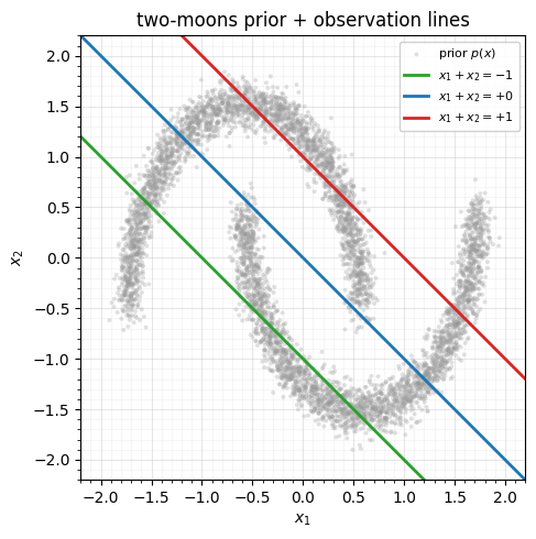
Each line is one observation. Where it crosses one crescent the posterior is a single blob; where it crosses both, the posterior is bimodal — watch the $y=0$ (anti-diagonal) line, which clips both moons.

2. Train the amortised posterior¶

A conditional coupling flow $p_\theta(x\mid y)$ (fixed $\mathcal{N}(0,I)$ base, RQSplineCoupling(cond_dim=1) reading the scalar observation) trained by NLL on the simulated pairs. One run; the posterior for every $y$ comes for free afterwards.

def make_flow(key, n_layers=6):
    keys = jr.split(key, n_layers)
    perm = jnp.array([1, 0])
    tr = []
    for i, k in enumerate(keys):
        tr.append(RQSplineCoupling(k, shape=(2,), n_bins=8, interval=5.0,
                                   cond_dim=1, nn_width=64, nn_depth=2))
        if i < n_layers - 1:
            tr.append(Permute(perm))
    return Transformed(Normal(jnp.zeros(2)), Chain(tr))


steps = -(-int(X.shape[0] * 0.9) // 256)
lr = optax.cosine_decay_schedule(3e-3, decay_steps=350 * steps, alpha=0.02)
opt = optax.chain(optax.clip_by_global_norm(5.0), optax.adam(lr))
post, losses = fit_to_data(jr.key(1), make_flow(jr.key(2)), (X, Y), optimizer=opt,
                           max_epochs=350, max_patience=350, batch_size=256,
                           val_prop=0.1, show_progress=False)
print(f"trained amortised posterior: {len(losses['train'])} epochs, "
      f"val NLL {float(min(losses['val'])):+.4f}")

trained amortised posterior: 350 epochs, val NLL -0.8465

3. The amortised posterior vs a rejection reference¶

For each observation $y$ we compare two posteriors. The reference is rejection sampling on the prior — keep prior draws whose $Ax$ falls within a hair of $y$ — which is exact but throws away almost every sample. The flow posterior is one batched sample(condition=y) call. They should agree, and the flow should recover the bimodal $y=0$ case.

def reject_posterior(key, yv, tol=0.06, n_keep=1500):
    big = prior(key, 300000)
    resid = jnp.abs((big @ A.T)[:, 0] - yv)
    return big[resid < tol][:n_keep]


def flow_posterior(yv, n, key):
    c = jnp.array([yv])
    return jax.vmap(lambda k: post.sample(k, condition=c))(jr.split(key, n))


fig, axes = plt.subplots(1, 3, figsize=(15, 5.2), sharex=True, sharey=True)
xs = np.linspace(-2.5, 2.5, 10)
for ax, yv in zip(axes, y_demo):
    ref = reject_posterior(jr.fold_in(jr.key(5), int((yv + 2) * 10)), yv)
    fs = flow_posterior(yv, 1500, jr.fold_in(jr.key(6), int((yv + 2) * 10)))
    ax.scatter(np.asarray(X[:, 0]), np.asarray(X[:, 1]), s=6, alpha=0.12, color="0.7", edgecolors="none")
    ax.scatter(np.asarray(ref[:, 0]), np.asarray(ref[:, 1]), s=14, alpha=0.5, color=DATA_COLOR,
               edgecolors="none", label="rejection reference")
    ax.scatter(np.asarray(fs[:, 0]), np.asarray(fs[:, 1]), s=10, alpha=0.4, color="tab:red",
               edgecolors="none", label="flow posterior")
    ax.plot(xs, yv - xs, color="0.2", lw=1.2, ls="--")
    ax.set(title=f"$p(x \\mid y={yv:+.0f})$", xlabel="$x_1$", xlim=(-2.2, 2.2), ylim=(-2.2, 2.2))
    ax.set_aspect("equal"); style_ax(ax)
axes[0].set_ylabel("$x_2$")
axes[0].legend(loc="upper left", fontsize=8, framealpha=0.9)
fig.suptitle("Amortised posterior (red) vs rejection reference (blue), one trained flow", y=1.01)
fig.tight_layout()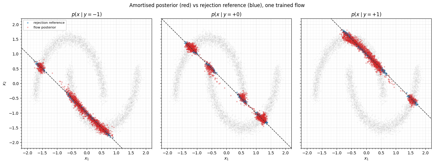

The flow posteriors sit on the moons, hug the observation line, and at $y=0$ the flow splits into two modes — one per crescent — matching the reference. All three come from the same network, evaluated at three different $y$ .

4. Observation consistency¶

A correct posterior must be consistent with the measurement: pushing posterior samples back through $A$ should recenter on the observed $y$ with spread $\approx\sigma$ . We histogram $A\hat x$ for the flow samples at each $y$ .

fig, axes = plt.subplots(1, 3, figsize=(15, 3.6), sharex=True, sharey=True)
for ax, yv in zip(axes, y_demo):
    fs = flow_posterior(yv, 4000, jr.fold_in(jr.key(8), int((yv + 2) * 10)))
    Ax = np.asarray((fs @ A.T)[:, 0])
    ax.hist(Ax, bins=45, density=True, color=LATENT_COLOR, alpha=0.8)
    ax.axvline(yv, color="tab:red", lw=2, label=f"observed $y={yv:+.0f}$")
    ax.set(title=f"$A\\hat x$ for flow posterior at $y={yv:+.0f}$", xlabel="$x_1+x_2$")
    ax.legend(fontsize=8); style_ax(ax)
    print(f"y={yv:+.0f}:  mean(Ax)={Ax.mean():+.3f} (target {yv:+.1f}),  std(Ax)={Ax.std():.3f} (target {SIGMA})")
axes[0].set_ylabel("density")
fig.tight_layout()

y=-1:  mean(Ax)=-1.007 (target -1.0),  std(Ax)=0.099 (target 0.1)

y=+0:  mean(Ax)=+0.005 (target +0.0),  std(Ax)=0.105 (target 0.1)

y=+1:  mean(Ax)=+0.993 (target +1.0),  std(Ax)=0.103 (target 0.1)

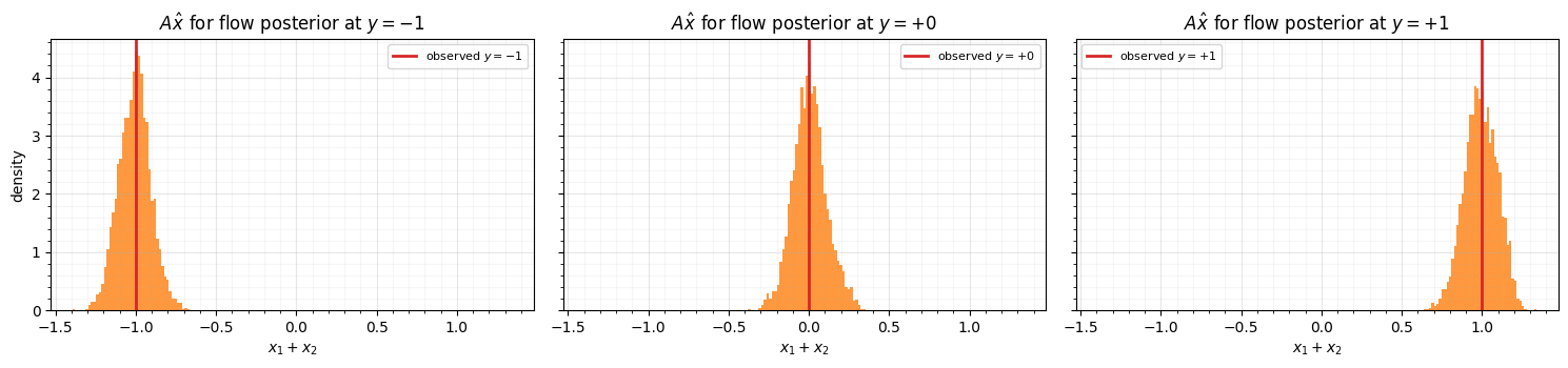
The reprojected samples center on $y$ with standard deviation close to the noise σ — the flow learned the likelihood, not just the prior support.

Recap — and the end of Part 7¶

	amortised flow posterior (here)	classical inversion
cost per new $y$	one forward pass	an optimisation / MCMC run
training	once, on simulated $(x,y)$	none (but solve every time)
multimodal posteriors	yes, by construction	needs many restarts / chains
needs the forward model	only to simulate pairs	explicitly, every solve

A conditional flow turns inference into amortisation: simulate $(x, y=Ax+\eta)$ , fit $p_\theta(x\mid y)$ once, and read off the posterior — bimodal and all — for any observation in a single pass. This closes Part 7: from where to inject context (00), through conditional density estimation and the marginals-vs-couplings rule (01), to conditioning on an observation for inverse problems.

Where this goes next. When the prior is itself a (Gaussianization) flow rather than something we can simulate from cheaply, the amortised route is replaced by a plug-and-play scheme that alternates a data-fit step with the flow prior’s closed-form proximal/Gaussianization step — the subject of Part 16. The toy here is the amortised counterpart of those solvers.

References¶

Papamakarios, G., Nalisnick, E., Rezende, D. J., Mohamed, S., & Lakshminarayanan, B. (2021). Normalizing Flows for Probabilistic Modeling and Inference. Journal of Machine Learning Research, 22(57), 1–64.
Winkler, C., Worrall, D. E., Hoogeboom, E., & Welling, M. (2019). Learning Likelihoods with Conditional Normalizing Flows. arXiv Preprint arXiv:1912.00042.