Conditional marginals & density estimation

01 — Conditional marginals & density estimation¶

In 00 the context was a discrete class label. The more common case is a continuous context $y$ : a covariate, a sensor setting, a forcing. The conditional flow then estimates a whole curve of densities $p(x\mid y)$ , with the usual conditional change of variables

p(x\mid y) = p_Z\big(T_\theta(x; y)\big)\,\big|\det J_{T_\theta(\cdot;y)}(x)\big|,

((1))

and — keeping a fixed $\mathcal{N}(0,I)$ base — the map $T_\theta(\cdot\mid y)$ is a genuine conditional Gaussianizer: every slice $p(x\mid y)$ is carried to the same standard normal. That gives us back the diagnostic notebook 00 had to skip: push a slice’s data through $T_\theta(\cdot\mid y)$ and check it lands on $\mathcal{N}(0,I)$ .

The other question this notebook answers is 7.2 — when do you condition the marginals versus the couplings? A conditional marginal makes each coordinate’s CDF depend on $y$ — cheap, and enough when the coordinates are conditionally independent given $y$ . The moment $y$ induces dependence between coordinates, only a conditional coupling can follow it. We make that concrete on a family that bends.

What you will see

A 2-D conditional $p(x\mid y)$ that morphs with a continuous $y$ .
The learned density and samples swept across $y$ .
The Gaussianization check: each slice $T_\theta(\cdot\mid y)$ -maps to $\mathcal{N}(0,I)$ .
Couplings vs marginals: the marginal/diagonal model captures spread but cannot bend — the rule of thumb for 7.2.

import warnings

warnings.filterwarnings("ignore")

import equinox as eqx
import jax
import jax.numpy as jnp
import jax.random as jr
import matplotlib.pyplot as plt
import numpy as np
import optax
from flowjax.bijections import Chain, Permute
from flowjax.distributions import Normal, Transformed
from flowjax.train import fit_to_data
from scipy import stats

from gauss_flows import ConditionalDiagGaussian, RQSplineCoupling, RQSplineMarginal
from _style import DATA_COLOR, GAUSS_KW, LATENT_COLOR, SCATTER_KW, style_ax

jax.config.update("jax_enable_x64", True)

1. A conditional family that bends¶

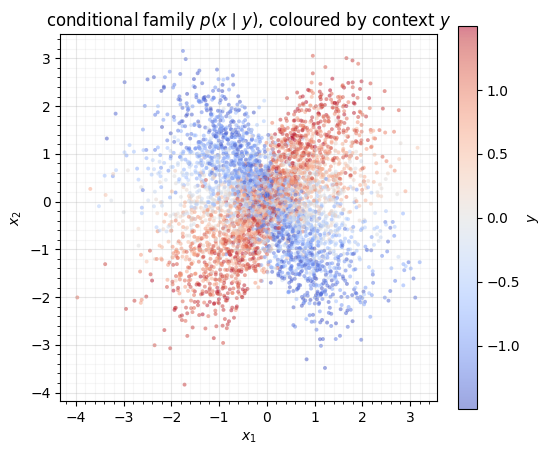
Draw $u\sim\mathcal{N}(0,I_2)$ and set $x_1 = 0.8\,u_1$ , $x_2 = 0.6\,u_2 + 1.5\,y\,\tanh(1.2\,u_1)$ . The context $y$ controls an S-shaped tilt: at $y=0$ the two coordinates are independent ( $x_2$ is just noise); as $|y|$ grows $x_2$ rises with $x_1$ for $y>0$ and falls for $y<0$ , tilting and bending the cloud. So $y$ changes both the shape of $p(x\mid y)$ and the dependence between $x_1$ and $x_2$ — while the $\tanh$ keeps tails bounded (a raw $u_1^2$ bend blows the spline’s support). We standardise $x$ with fixed stats.

Y_LO, Y_HI = -1.5, 1.5


def sample_banana(key, n, y_fixed=None):
    ku, ky = jr.split(key)
    y = (jnp.full((n, 1), y_fixed) if y_fixed is not None
         else jr.uniform(ky, (n, 1), minval=Y_LO, maxval=Y_HI))
    u = jr.normal(ku, (n, 2))
    x1 = 0.8 * u[:, 0]
    x2 = 0.6 * u[:, 1] + 1.5 * y[:, 0] * jnp.tanh(1.2 * u[:, 0])
    return jnp.stack([x1, x2], -1), y


# Fixed standardisation stats from a large pilot sample.
_pilot, _ = sample_banana(jr.key(99), 20000)
X_MEAN, X_STD = _pilot.mean(0), _pilot.std(0)


def dataset(key, n, y_fixed=None):
    x, y = sample_banana(key, n, y_fixed)
    return (x - X_MEAN) / X_STD, y


X, Y = dataset(jr.key(0), 5000)
print(f"X {X.shape}, context Y {Y.shape}, y in [{Y_LO}, {Y_HI}]  (standardised x)")

# colour the cloud by y to show the morphing family in one panel
fig, ax = plt.subplots(figsize=(5.6, 5))
sc = ax.scatter(np.asarray(X[:, 0]), np.asarray(X[:, 1]), c=np.asarray(Y[:, 0]),
                cmap="coolwarm", s=8, alpha=0.5, edgecolors="none")
ax.set(title="conditional family $p(x\\mid y)$, coloured by context $y$",
       xlabel="$x_1$", ylabel="$x_2$")
ax.set_aspect("equal"); style_ax(ax)
fig.colorbar(sc, ax=ax, label="$y$", fraction=0.046)
fig.tight_layout()

X (5000, 2), context Y (5000, 1), y in [-1.5, 1.5]  (standardised x)

2. A couplings-conditioned flow¶

A fixed $\mathcal{N}(0,I)$ base plus a chain of RQSplineCoupling(cond_dim=1) layers (the context $y$ is concatenated into each conditioner) with Permutes between them. Built as a flowjax Transformed so we can call chain.inverse(x, y) — the Gaussianization map — directly. We train by conditional NLL.

def make_coupling_flow(key, n_layers=5):
    keys = jr.split(key, n_layers)
    perm = jnp.array([1, 0])
    transforms = []
    for i, k in enumerate(keys):
        transforms.append(RQSplineCoupling(k, shape=(2,), n_bins=8, interval=5.0,
                                           cond_dim=1, nn_width=64, nn_depth=2))
        if i < n_layers - 1:
            transforms.append(Permute(perm))
    return Transformed(Normal(jnp.zeros(2)), Chain(transforms))


def train(dist, key, max_epochs=300):
    steps = -(-int(X.shape[0] * 0.9) // 256)
    lr = optax.cosine_decay_schedule(3e-3, decay_steps=max_epochs * steps, alpha=0.02)
    opt = optax.chain(optax.clip_by_global_norm(5.0), optax.adam(lr))
    trained, losses = fit_to_data(key, dist, (X, Y), optimizer=opt, max_epochs=max_epochs,
                                  max_patience=max_epochs, batch_size=256, val_prop=0.1,
                                  show_progress=False)
    return trained, losses


cpl, cpl_losses = train(make_coupling_flow(jr.key(1)), jr.key(2))
print(f"coupling flow: {len(cpl_losses['train'])} epochs, val NLL {float(min(cpl_losses['val'])):+.4f}")

coupling flow: 300 epochs, val NLL +2.2626

3. The learned density, swept across the context¶

The point of a conditional model: one trained flow gives $p(x\mid y)$ for any $y$ . Top row — true data sampled at each $y$ ; bottom row — the flow’s density on a grid at the same $y$ . The learned banana bends the right way and by the right amount as $y$ moves from -1.2 to +1.2.

y_slices = jnp.array([-1.2, -0.6, 0.0, 0.6, 1.2])
lim, gn = 3.5, 70
xs = jnp.linspace(-lim, lim, gn)
gx, gy = jnp.meshgrid(xs, xs)
grid = jnp.stack([gx.ravel(), gy.ravel()], -1)


@eqx.filter_jit
def density_at(dist, yv):
    c = jnp.array([yv])  # context is the raw y value
    return jnp.exp(jax.vmap(lambda p: dist.log_prob(p, condition=c))(grid)).reshape(gn, gn)


fig, axes = plt.subplots(2, len(y_slices), figsize=(15, 6.2), sharex=True, sharey=True)
for j, yv in enumerate(y_slices):
    xt, _ = dataset(jr.fold_in(jr.key(7), j), 1500, y_fixed=float(yv))
    axes[0, j].scatter(np.asarray(xt[:, 0]), np.asarray(xt[:, 1]), color=DATA_COLOR, **SCATTER_KW)
    axes[0, j].set(title=f"$y={float(yv):+.1f}$", xlim=(-lim, lim), ylim=(-lim, lim))
    axes[1, j].contourf(np.asarray(gx), np.asarray(gy), np.asarray(density_at(cpl, float(yv))),
                        levels=18, cmap="viridis")
    for r in (0, 1):
        axes[r, j].set_aspect("equal"); style_ax(axes[r, j])
axes[0, 0].set_ylabel("true data")
axes[1, 0].set_ylabel("learned $p(x\\mid y)$")
fig.suptitle("Conditional density swept across the context $y$", y=1.01)
fig.tight_layout()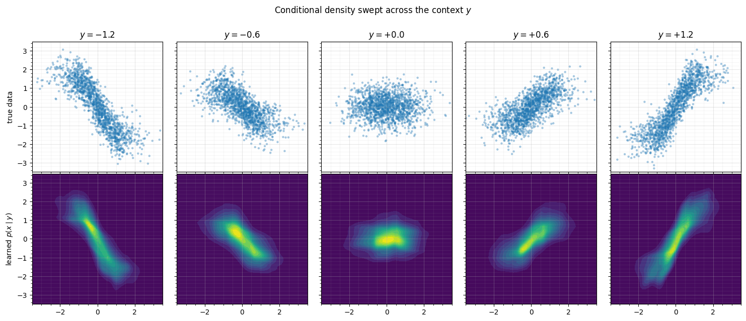

4. The Gaussianization check¶

Because the base is a fixed $\mathcal{N}(0,I)$ , the map $T_\theta(\cdot\mid y) =$ chain.inverse(x, y) should send every slice to the same standard normal. We push each slice’s data through it and look: the conditional bananas all collapse onto the $\mathcal{N}(0,I)$ rings, with moments near $(0,1,0,0)$ regardless of $y$ .

chain = cpl.bijection
th = np.linspace(0, 2 * np.pi, 200)
check_ys = [-1.0, 0.0, 1.0]
fig, axes = plt.subplots(1, 3, figsize=(14.5, 4.8), sharex=True, sharey=True)
print("Gaussianized-slice moments (target 0, 1, 0, 0):")
for ax, yv in zip(axes, check_ys):
    xt, _ = dataset(jr.fold_in(jr.key(13), int((yv + 2) * 10)), 1500, y_fixed=yv)
    c = jnp.array([yv])
    z = np.asarray(jax.vmap(lambda p: chain.inverse(p, condition=c))(xt))
    ax.scatter(z[:, 0], z[:, 1], color=LATENT_COLOR, **SCATTER_KW)
    for r in (1.0, 2.0):
        ax.plot(r * np.cos(th), r * np.sin(th), **GAUSS_KW)
    ax.set(title=f"$z = T(x\\mid y={yv:+.0f})$", xlabel="$z_1$", xlim=(-3.6, 3.6), ylim=(-3.6, 3.6))
    ax.set_aspect("equal"); style_ax(ax)
    print(f"  y={yv:+.0f}: mean=({z[:,0].mean():+.2f},{z[:,1].mean():+.2f})  "
          f"std=({z[:,0].std():.2f},{z[:,1].std():.2f})  "
          f"exc-kurt=({stats.kurtosis(z[:,0]):+.2f},{stats.kurtosis(z[:,1]):+.2f})")
axes[0].set_ylabel("$z_2$")
fig.suptitle(r"Every conditional slice Gaussianizes to the same $\mathcal{N}(0,I)$", y=1.02)
fig.tight_layout()

Gaussianized-slice moments (target 0, 1, 0, 0):

  y=-1: mean=(+0.10,+0.06)  std=(0.99,0.89)  exc-kurt=(-0.20,-0.33)

  y=+0: mean=(-0.09,-0.03)  std=(1.00,0.90)  exc-kurt=(-0.05,-0.07)

  y=+1: mean=(-0.08,+0.01)  std=(1.06,0.92)  exc-kurt=(+0.10,-0.03)

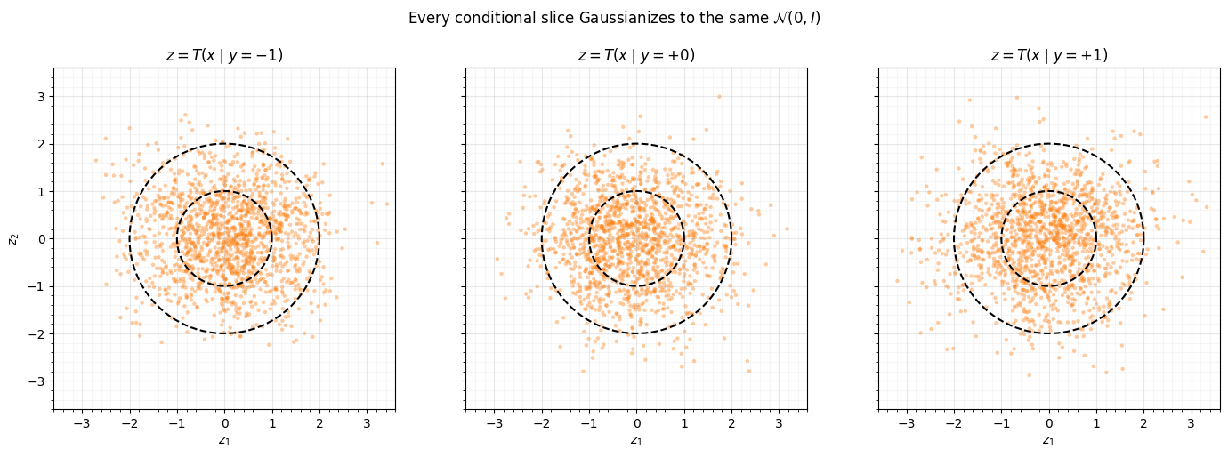
Three different bananas, one standard normal — that is the conditional Gaussianizer working. (Compare notebook 00, where SurVAEFlow did not expose this forward map; a flowjax Transformed does.)

5. When do y-dependent marginals suffice? (7.2)¶

A cheaper option conditions only the margins — here a ConditionalDiagGaussian base (per-coordinate $y$ -dependent location/scale) with unconditional spline margins and no coupling. Such a model can stretch and shift each axis with $y$ , but it treats the coordinates as independent given $y$ , so it cannot represent the banana’s $y$ -induced dependence. We fit it and compare.

def make_diagonal_flow(key, n_layers=3):
    base = ConditionalDiagGaussian(key, event_shape=(2,), cond_shape=(1,))
    margins = [RQSplineMarginal(n_bins=8, shape=(2,), interval=5.0) for _ in range(n_layers)]
    return Transformed(base, Chain(margins))


diag, diag_losses = train(make_diagonal_flow(jr.key(3)), jr.key(4))


def mean_nll(dist):
    f = eqx.filter_jit(lambda x, c: jax.vmap(lambda xi, ci: dist.log_prob(xi, condition=ci))(x, c))
    return -float(jnp.mean(f(X, Y)))


print(f"\nmean conditional NLL (lower is better):")
print(f"  marginal / diagonal (y -> base only): {mean_nll(diag):+.4f}")
print(f"  coupling (y -> couplings)           : {mean_nll(cpl):+.4f}")

yv = 1.2
xt, _ = dataset(jr.key(21), 1500, y_fixed=yv)
fig, axes = plt.subplots(1, 3, figsize=(14.5, 4.8), sharex=True, sharey=True)
axes[0].scatter(np.asarray(xt[:, 0]), np.asarray(xt[:, 1]), color=DATA_COLOR, **SCATTER_KW)
axes[0].set(title=f"true data, $y={yv}$")
axes[1].contourf(np.asarray(gx), np.asarray(gy), np.asarray(density_at(diag, yv)), levels=18, cmap="viridis")
axes[1].set(title="marginal / diagonal $p(x\\mid y)$\n(cannot bend)")
axes[2].contourf(np.asarray(gx), np.asarray(gy), np.asarray(density_at(cpl, yv)), levels=18, cmap="viridis")
axes[2].set(title="coupling $p(x\\mid y)$\n(follows the bend)")
for ax in axes:
    ax.set(xlim=(-lim, lim), ylim=(-lim, lim), xlabel="$x_1$")
    ax.set_aspect("equal"); style_ax(ax)
axes[0].set_ylabel("$x_2$")
fig.tight_layout()


mean conditional NLL (lower is better):

  marginal / diagonal (y -> base only): +2.7301

  coupling (y -> couplings)           : +2.2395

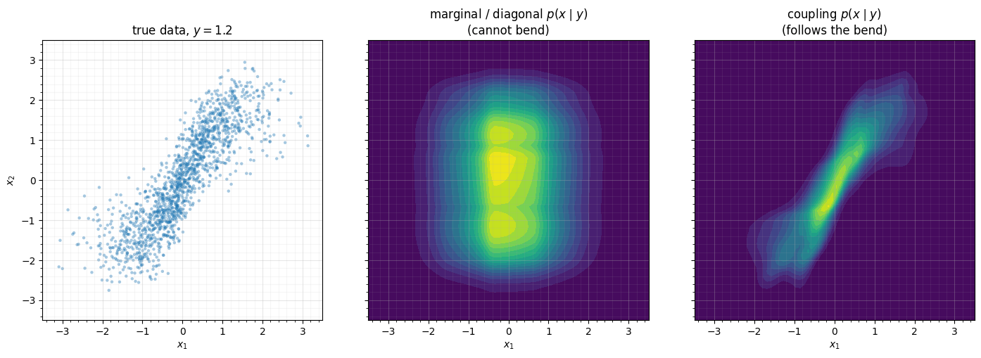
The diagonal model widens $x_2$ as $|y|$ grows — it sees the marginal spread — but its density stays an axis-aligned blob, because no elementwise margin can make $x_2$ depend on $x_1$ . The coupling flow bends with the data and wins on NLL.

Recap¶

$y$ changes...	enough to condition...	why
per-coordinate location / scale	marginals (or the base)	coordinates stay independent given $y$
per-coordinate shape (skew, tails)	marginals (richer CDF)	still elementwise
the dependence between coordinates	couplings (`cond_dim`)	only a coupling reads one coordinate to transform another

So: reach for conditional marginals when $y$ only reshapes each axis, and for conditional couplings the moment $y$ couples the axes — which the banana does. With a fixed $\mathcal{N}(0,I)$ base, the trained coupling flow is a conditional Gaussianizer that maps every slice $p(x\mid y)$ to the same standard normal, as the check in §4 confirmed.

Next up. 02 — Conditional flow as an amortised posterior turns the context into an observation $y = Ax + \eta$ and trains $p(x\mid y)$ as a one-pass posterior for an inverse problem — the bridge to the plug-and-play priors of Part 16.