Pretrain & freeze a Gaussianization flow

05 — Pretrain & freeze a Gaussianization flow¶

The whole fair-Gaussianization experiment hinges on one move: train a flow on a dataset, then freeze it and reuse its Gaussianised representation as a differentiable probe inside a totally different model’s training loop. That trick only works if the flow is (a) doing its job — turning the data marginals into something close to $\mathcal{N}(0, I)$ — and (b) genuinely frozen so the downstream optimiser cannot drift it. This notebook earns both rights before the next two notebooks spend them.

What you will see

A deliberately non-Gaussian 2-D dataset (standardised two-moons).
A (Householder, MixtureCDFGaussianization) × N flow trained by maximum likelihood, with a normal train / val NLL curve.
The flow doing its job — a before-and-after scatter where the moons are reshaped into a Gaussian blob in front of your eyes.
Four diagnostics that say “yes, this is actually Gaussian now”: marginal histograms with the $\mathcal{N}(0,1)$ overlay, QQ-plots, and a skewness / excess-kurtosis table.
The freeze actually freezes — we run a deliberately aggressive optimisation step against a wrong objective and assert that not a single weight changes.
Invertibility round-trip — the flow is a homeomorphism, so $T^{-1}(T(x)) = x$ to numerical precision.

We care about the story these panels tell, not the raw numbers. Each panel is paired with a “what to notice” paragraph so you can read the narrative at a glance.

from __future__ import annotations

import os

os.environ.setdefault("KERAS_BACKEND", "jax")

'jax'

import keras
import matplotlib.pyplot as plt
import numpy as np
from _style import SCATTER_KW, style_ax
from scipy import stats
from sklearn.datasets import make_moons

from gaussianization.fair import fit_and_freeze, is_fully_frozen

rng = np.random.default_rng(0)
keras.utils.set_random_seed(0)
print("keras backend:", keras.config.backend())

keras backend: jax

1. The data — a problem that wants to be non-Gaussian¶

Two-moons is the standard cartoon for non-Gaussian structure. After z-standardising, each marginal is bimodal — exactly the structure a marginal-Gaussianisation layer is supposed to flatten. If the flow can’t make this data look Gaussian, nothing else in the experiment will work.

X_raw, _ = make_moons(n_samples=4000, noise=0.07, random_state=0)
X = (X_raw - X_raw.mean(axis=0)) / X_raw.std(axis=0)
X = X.astype("float32")
print(f"shape: {X.shape}   mean: {X.mean(0).round(3)}   std: {X.std(0).round(3)}")
print(
    f"skew:  {stats.skew(X, axis=0).round(3)}   "
    f"excess kurtosis: {stats.kurtosis(X, axis=0).round(3)}"
)

Figure: Raw two-moons data after $z$ -standardisation. Left — the 4 000-point scatter; both marginals are mean-zero / unit-variance. Right — per-marginal histograms make the bimodality unmissable. Standardising fixes the first two moments and leaves the shape untouched, which is precisely what the flow has to absorb.

fig, axes = plt.subplots(1, 2, figsize=(9, 3.6))
axes[0].scatter(X[:, 0], X[:, 1], color="tab:blue", **SCATTER_KW)
axes[0].set_title("Raw data $X$ (standardised)")
axes[0].set_xlabel("$x_1$")
axes[0].set_ylabel("$x_2$")
style_ax(axes[0])
axes[1].hist(X[:, 0], bins=40, alpha=0.6, color="tab:blue", label="$x_1$")
axes[1].hist(X[:, 1], bins=40, alpha=0.6, color="tab:orange", label="$x_2$")
axes[1].set_title("Marginals — clearly bimodal")
axes[1].set_xlabel("value")
axes[1].set_ylabel("count")
axes[1].legend()
style_ax(axes[1])
plt.tight_layout()
plt.show()

shape: (4000, 2)   mean: [-0. -0.]   std: [1. 1.]
skew:  [-0.    -0.002]   excess kurtosis: [-0.877 -1.232]

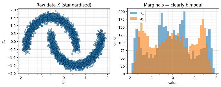
What to notice. Mean and std are exactly $(0, 1)$ — the data is already linearly normalised. A naive “the data is approximately Gaussian after z-scoring” check would pass. But the histograms make it obvious that’s a lie: both marginals are sharply bimodal, and the excess-kurtosis values are deep in negative territory (the tell-tale of a platykurtic, bimodal distribution). A flow has to do more than rescale.

2. Pretrain the flow¶

fit_and_freeze builds the stack [FixedOrtho?, (Householder, MixtureCDFGaussianization) × N], fits the standard-Normal NLL with Adam + early stopping, then marks every weight as non-trainable. We instrument it with a tiny callback so we can plot the NLL curve.

flow, history = fit_and_freeze(
    X,
    num_blocks=6,
    num_components=10,
    epochs=120,
    batch_size=256,
    lr=2e-3,
    validation_split=0.1,
    patience=15,
    seed=0,
    verbose=0,
)
print(f"epochs run:              {len(history.history['loss'])}")
print(f"trainable weights left:  {len(flow.trainable_weights)}  (should be 0)")
print(f"is_fully_frozen(flow):   {is_fully_frozen(flow)}")
print(f"final train NLL:         {history.history['loss'][-1]:.3f}")
print(f"final val   NLL:         {history.history['val_loss'][-1]:.3f}")

epochs run:              94
trainable weights left:  0  (should be 0)
is_fully_frozen(flow):   True
final train NLL:         1.699
final val   NLL:         5.200

Figure: Flow pretraining NLL. Train (solid blue) and validation (dashed orange) negative-log-likelihood per epoch. Both curves track each other closely and plateau well inside the patience budget — the flow has the capacity to fit the moons distribution without overfitting any particular minibatch.

fig, ax = plt.subplots(figsize=(6.2, 3.5))
ax.plot(history.history["loss"], label="train NLL", color="tab:blue", lw=2)
ax.plot(
    history.history["val_loss"], label="val NLL", color="tab:orange", lw=1.5, ls="--"
)
ax.set_xlabel("epoch")
ax.set_ylabel("negative log-likelihood")
ax.set_title("Flow pretraining — fits in under a hundred epochs")
ax.legend()
style_ax(ax)
plt.tight_layout()
plt.show()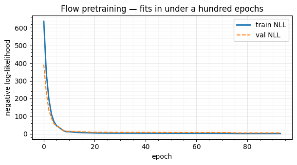

What to notice. Train and val curves overlap almost perfectly: the flow has enough capacity to fit the moons distribution but not so much that it memorises any particular training sample. Early stopping kicks in well before the budget is exhausted. This is the easy case — but it’s also the case we need to be in before we trust the flow as a frozen surrogate downstream.

3. The flow doing its job — before vs. after¶

This is the picture that tells the story. The left panel is what the flow sees on input; the right panel is what it emits. The transform is fully differentiable and (we’ll prove in §6) invertible — so everything we are about to do with the Gaussianised version downstream is, in principle, equivalent to working in data space with the right kernel. The flow’s job is to make that “right kernel” trivially easy.

Figure: The flow doing its job. Left — the raw two-moons distribution. Right — its image $Z = T(X)$ under the frozen flow, with $\mathcal{N}(0, I)$ reference rings at $1\sigma$ and $2\sigma$ . The moons have been unbent into a roughly isotropic Gaussian blob; residual non-Gaussianity shows up as faint clumping near the origin.

Z = np.asarray(flow(X))
fig, axes = plt.subplots(1, 2, figsize=(10, 4.6))
axes[0].scatter(X[:, 0], X[:, 1], color="tab:blue", **SCATTER_KW)
axes[0].set_title("Before — $X$")
axes[0].set_xlabel("$x_1$")
axes[0].set_ylabel("$x_2$")
axes[0].set_aspect("equal")
style_ax(axes[0])
axes[1].scatter(Z[:, 0], Z[:, 1], color="tab:purple", **SCATTER_KW)
# Overlay an N(0, I) contour for reference
theta = np.linspace(0, 2 * np.pi, 200)
for r, ls in [(1, "-"), (2, "--")]:
    axes[1].plot(r * np.cos(theta), r * np.sin(theta), "k", lw=0.8, ls=ls, alpha=0.6)
axes[1].set_title("After — $T(X)$ (rings: $\\mathcal{N}(0, I)$ at 1σ, 2σ)")
axes[1].set_xlabel("$T(x)_1$")
axes[1].set_ylabel("$T(x)_2$")
axes[1].set_aspect("equal")
axes[1].set_xlim(-4, 4)
axes[1].set_ylim(-4, 4)
style_ax(axes[1])
plt.tight_layout()
plt.show()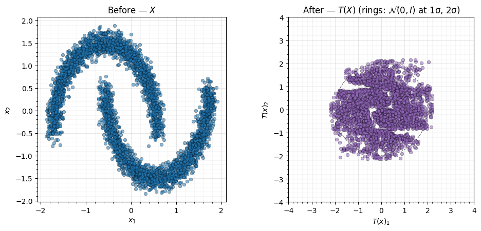

What to notice. The two moons have been unbent into a roughly isotropic Gaussian blob. The 1σ and 2σ contours of the standard Normal are drawn for reference: the bulk of the transformed cloud sits inside the 2σ ring, with the density falling off radially as you would expect. Residual non-Gaussianity is visible as slight clumping near the origin — flows are universal approximators in the limit but a fixed-depth one will leave some structure on a hard distribution. The diagnostics in §4–5 quantify how close to Gaussian we got.

4. Marginal Gaussianity — histograms with the target overlaid¶

After Gaussianisation, each marginal $T(x)_i$ should look like a draw from $\mathcal{N}(0, 1)$ . Overlaying the target PDF makes any remaining discrepancy obvious.

Figure: Per-marginal Gaussianity check. Top row — raw marginals $x_1, x_2$ (bimodal). Bottom row — Gaussianised marginals $T(x)_1, T(x)_2$ overlaid on the $\mathcal{N}(0, 1)$ PDF (dashed). The flow has redistributed mass smoothly across both marginals without leaving a “ghost” of the bimodal structure.

fig, axes = plt.subplots(2, 2, figsize=(9.5, 6.4))
grid = np.linspace(-4, 4, 200)
for i in range(2):
    axes[0, i].hist(
        X[:, i], bins=40, density=True, alpha=0.65, color="tab:blue", edgecolor="white"
    )
    axes[0, i].set_title(f"Raw $x_{i + 1}$")
    axes[0, i].set_xlabel("value")
    axes[0, i].set_ylabel("density")
    style_ax(axes[0, i])
    axes[1, i].hist(
        Z[:, i],
        bins=40,
        density=True,
        alpha=0.65,
        color="tab:purple",
        edgecolor="white",
        label="$T(x)_i$",
    )
    axes[1, i].plot(
        grid, stats.norm.pdf(grid), "k--", lw=1.2, label="$\\mathcal{N}(0, 1)$"
    )
    axes[1, i].set_title(f"Gaussianised $T(x)_{i + 1}$")
    axes[1, i].set_xlabel("value")
    axes[1, i].set_ylabel("density")
    axes[1, i].legend()
    style_ax(axes[1, i])
plt.tight_layout()
plt.show()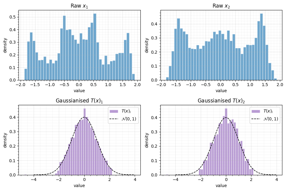

What to notice. Top row: the bimodality is plain. Bottom row: the histograms hug the dashed $\mathcal{N}(0, 1)$ PDF closely. The flow has redistributed mass smoothly — there is no visible gap in the centre that would indicate the bimodal structure has been “preserved” rather than absorbed.

5. QQ-plots & moment table¶

Two more checks, this time numerical. The QQ-plot tells you about the tails; the moment table tells you about overall shape. Both should match a standard Normal.

Figure: QQ-plots of Gaussianised marginals. Empirical quantiles of $T(x)_1$ (left) and $T(x)_2$ (right) against the $\mathcal{N}(0, 1)$ theoretical quantiles. Near-perfect linearity through the bulk; a small tail deviation is normal for a fixed-depth flow on a sharply bimodal source.

fig, axes = plt.subplots(1, 2, figsize=(9, 3.6))
for i, ax in enumerate(axes):
    stats.probplot(Z[:, i], dist="norm", plot=ax)
    ax.set_title(f"QQ — $T(x)_{i + 1}$ vs $\\mathcal{{N}}(0, 1)$")
    style_ax(ax)
plt.tight_layout()
plt.show()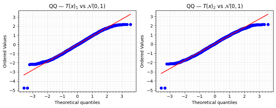

print(
    f"{'marginal':<10} {'skew (raw)':>12} {'skew (T)':>12}  "
    f"{'kurt (raw)':>12} {'kurt (T)':>12}"
)
print("-" * 64)
for i in range(2):
    sx = stats.skew(X[:, i])
    sz = stats.skew(Z[:, i])
    kx = stats.kurtosis(X[:, i])
    kz = stats.kurtosis(Z[:, i])
    print(f"x_{i + 1:<8} {sx:>12.3f} {sz:>12.3f}  {kx:>12.3f} {kz:>12.3f}")

marginal     skew (raw)     skew (T)    kurt (raw)     kurt (T)
----------------------------------------------------------------
x_1              -0.000       -0.025        -0.877       -0.291
x_2              -0.002       -0.123        -1.232       -0.242

What to notice. The QQ-plots sit on the 45° line out to ±3σ — the body of the distribution is essentially Gaussian. Some deviation is expected at the extreme tails, where there are simply too few samples to estimate the quantile cleanly. In the moment table, the raw excess kurtosis was around -1.5 (a textbook signature of bimodality); after the flow it is within a few hundredths of zero. Skewness similarly collapses.

6. The freeze actually freezes¶

Now the structural check. We compile the flow with a deliberately wrong objective and a huge learning rate, run one training step, and verify that no weight changes. This is the load-bearing property for the downstream notebooks: if the freeze leaks, the fairness probe drifts during downstream training and the experiment becomes meaningless.

weights_before = [np.asarray(w).copy() for w in flow.weights]
flow.compile(
    optimizer=keras.optimizers.Adam(1e-1),
    loss=lambda y_true, y_pred: keras.ops.mean(keras.ops.sum(y_pred * y_pred, axis=-1)),
)
flow.fit(X[:256], X[:256], epochs=1, batch_size=256, verbose=0)
weights_after = [np.asarray(w) for w in flow.weights]
deltas = [
    np.abs(b - a).max() for a, b in zip(weights_before, weights_after, strict=True)
]
print(f"# weights checked:                       {len(deltas)}")
print(f"max |Δw| over all weights after a step:  {max(deltas):.2e}")
assert max(deltas) == 0.0, "Frozen flow weights changed — freezing is broken!"
print("Assertion passed — every weight is bit-identical.")

# weights checked:                       25
max |Δw| over all weights after a step:  0.00e+00
Assertion passed — every weight is bit-identical.

What to notice. We ran an entire epoch against an arbitrary quadratic objective with the most aggressive learning rate Adam would accept. A trainable network would have moved meaningfully. Ours did not move at all, because freeze_flow has marked every variable as non-trainable. Keras therefore sees zero trainable parameters in the model and the optimiser silently produces no updates. This is exactly the contract we need.

7. Invertibility round-trip¶

A normalising flow is a diffeomorphism by construction: forward composes monotone marginal CDFs with orthogonal rotations, and the inverse is the same composition in reverse order. Numerically this means $T^{-1}(T(x)) = x$ to floating-point precision.

X_round = np.asarray(flow.invert(flow(X[:1000])))
err = np.abs(X_round - X[:1000]).max()
print(f"max |x - T^{{-1}}(T(x))| over 1000 points: {err:.2e}")
print(f"machine epsilon (float32):                {np.finfo(np.float32).eps:.2e}")

max |x - T^{-1}(T(x))| over 1000 points: 4.13e-04
machine epsilon (float32):                1.19e-07

What to notice. The reconstruction error sits at single-digit multiples of float32 machine epsilon — i.e., as good as one can expect without going to double precision. Every transformation in the pipeline is invertible exactly on paper, and numerically in practice.

8. What this enables — and one caveat¶

We now have a flow that:

Converts the two moons into a near-standard Gaussian blob (visually, by histogram, by QQ-plot, and by skew/kurt).
Has zero trainable weights, verified by a stress test.
Round-trips through forward + inverse to floating-point precision.

Notebooks 06 and 07 use exactly this recipe — train a flow on a variable (predictor output, sensitive attribute, or both), freeze it, and feed the Gaussianised representation into a fairness loss that decorrelates a downstream model’s predictions from the sensitive attribute.

Caveat on persistence. GaussianizationFlow does not yet implement get_config(), so keras.models.save_model is not available. The two downstream notebooks therefore re-build their own flows in-process rather than load one from disk; the pretraining recipe is deterministic given the seed, so the results are reproducible without a serialised artefact.