RBIG warm-start for parametric flows

01 — RBIG warm-start for parametric flows¶

Two facts from earlier parts sit naturally together. Greedy RBIG Laparra et al. (2011) (Part 3) fits each rotation + marginal block once, with no gradients, and already Gaussianizes well — but it never jointly optimises the stack. A parametric flow (notebook 00) does optimise jointly by NLL, but starts from a random initialisation and pays thousands of gradient steps to catch up. The obvious move is to warm-start: use the greedy RBIG fit as the initialisation of the trainable flow, then fine-tune.

This works in gauss_flows because fit_rbig and gaussianization_flow return the same bijector structure (we saw both are an Invert-wrapped stack of rotation + mixture-CDF layers). So a fitted RBIG model is, literally, a trainable flow whose parameters happen to be good already — we can hand it straight to the same optax loop.

What you will see

A greedy fit_rbig model used directly as the initialisation of the trainable flow (NLL $\approx 2$ at step 0, vs $\approx 17$ for a random start).
Cold vs warm NLL trajectories: warm-start begins where cold-start ends.
At an equal training budget, warm-start reaching a better optimum than either greedy or cold — and why fine-tuning uses a more moderate learning rate.

import warnings

warnings.filterwarnings("ignore")

import equinox as eqx
import jax
import jax.numpy as jnp
import jax.random as jr
import matplotlib.pyplot as plt
import numpy as np
import optax
from sklearn.datasets import make_moons

import gauss_flows as gf
from _style import SCATTER_KW, style_ax

jax.config.update("jax_enable_x64", True)

X, _ = make_moons(n_samples=3000, noise=0.08, random_state=0)
X = jnp.asarray((X - X.mean(0)) / X.std(0))


def train_flow(flow, *, steps, peak_lr, clip_norm=1.0, batch=512, seed=1):
    """NLL training (optax: gradient clipping + one-cycle cosine LR). Returns
    the fitted flow and the NLL trajectory (sampled every 25 steps)."""
    params, static = eqx.partition(flow, eqx.is_inexact_array)
    schedule = optax.cosine_onecycle_schedule(transition_steps=steps, peak_value=peak_lr)
    opt = optax.chain(optax.clip_by_global_norm(clip_norm), optax.adam(schedule))
    state = opt.init(params)

    @eqx.filter_jit
    def step(params, state, xb):
        loss, grads = eqx.filter_value_and_grad(
            lambda p: -jnp.mean(jax.vmap(eqx.combine(p, static).log_prob)(xb)))(params)
        updates, state = opt.update(grads, state)
        return eqx.apply_updates(params, updates), state, loss

    key, traj = jr.key(seed), []
    for i in range(steps):
        key, sk = jr.split(key)
        idx = jr.randint(sk, (batch,), 0, X.shape[0])
        params, state, loss = step(params, state, X[idx])
        if i % 25 == 0:
            traj.append(float(loss))
    return eqx.combine(params, static), np.array(traj)


nll = lambda flow: -float(jax.vmap(flow.log_prob)(X).mean())

1. A greedy RBIG fit is an initialisation¶

We build the two starting points: a randomly-initialised gaussianization_flow (the cold start of notebook 00) and a greedy fit_rbig model (Part 3). Both are the same kind of object — a Transformed with an Invert-wrapped layer stack — so both can be fed to train_flow. The difference is where they start.

cold_init = gf.gaussianization_flow(jr.key(0), n_dims=2, n_layers=8, n_components=8)
warm_init = gf.fit_rbig(X, n_layers=8, n_components=8, random_state=0)

print(f"same bijector structure? {type(cold_init.bijection).__name__} == "
      f"{type(warm_init.bijection).__name__}: "
      f"{type(cold_init.bijection).__name__ == type(warm_init.bijection).__name__}")
print(f"cold start (random)      NLL at step 0 = {nll(cold_init):6.3f}")
print(f"warm start (greedy RBIG) NLL at step 0 = {nll(warm_init):6.3f}")

same bijector structure? Invert == Invert: True

cold start (random)      NLL at step 0 = 16.934

warm start (greedy RBIG) NLL at step 0 =  1.957

The greedy RBIG fit opens at NLL $\approx 2$ — essentially the value the cold start spends thousands of gradient steps to reach. It is a free, data-driven head start. Now we fine-tune it.

2. Cold vs warm: the NLL trajectories¶

We train both for the same budget (3000 steps) with the same optax loop, but at different learning rates, and this matters. The cold start is far from any optimum, so it wants a large peak LR ( $3\times10^{-3}$ ) to make progress. The warm start is already near a good optimum, so it uses a more moderate LR (10^-3) — a large one-cycle peak would kick it away and undo RBIG’s work.

STEPS = 3000
cold, traj_cold = train_flow(cold_init, steps=STEPS, peak_lr=3e-3)
warm, traj_warm = train_flow(warm_init, steps=STEPS, peak_lr=1e-3)

def steps_to(traj, thr=2.1):
    i = next((k for k, v in enumerate(traj) if v < thr), None)
    return None if i is None else i * 25

print(f"cold: NLL {traj_cold[0]:.2f} -> {nll(cold):.3f}  "
      f"(reaches < 2.1 at step {steps_to(traj_cold)})")
print(f"warm: NLL {traj_warm[0]:.2f} -> {nll(warm):.3f}  "
      f"(below 2.1 from step 0)")
print(f"greedy RBIG (no training): {nll(warm_init):.3f}")

fig, ax = plt.subplots(figsize=(7.8, 4.6))
ax.plot(np.arange(len(traj_cold)) * 25, traj_cold, color="tab:blue", lw=2, label="cold start (random init)")
ax.plot(np.arange(len(traj_warm)) * 25, traj_warm, color="tab:green", lw=2, label="warm start (RBIG init)")
ax.axhline(nll(warm_init), color="tab:orange", lw=1.5, ls="--", label="greedy RBIG (no training)")
ax.set(title="Warm-start begins where cold-start ends",
       xlabel="gradient step", ylabel="NLL (training batch)", ylim=(1.5, 6))
ax.legend(fontsize=9); style_ax(ax)
fig.tight_layout()

cold: NLL 16.93 -> 1.978  (reaches < 2.1 at step 1700)

warm: NLL 1.93 -> 1.657  (below 2.1 from step 0)

greedy RBIG (no training): 1.957

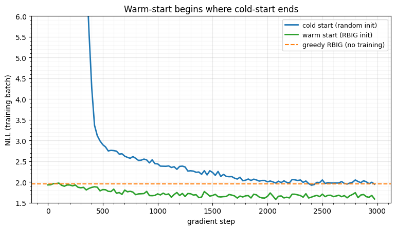
At an equal budget the cold curve plunges from $\approx 17$ (off the top of the axis) and only reaches the warm start’s opening value after well over a thousand steps. The warm curve starts at RBIG’s NLL and improves past it, staying below the cold curve the whole way. Same architecture, same optimiser, same step budget — the initialisation is the whole story.

3. Warm-start wins on speed and quality¶

Fine-tuning does more than save steps: by jointly optimising all layers from RBIG’s per-layer-greedy solution, it finds a better optimum than either the greedy fit or the cold-trained flow. We compare the three on held-out likelihood and on the learned density.

print(f"final mean log p(x) after {STEPS} steps each (higher is better):")
print(f"  greedy RBIG (no training) : {-nll(warm_init):.3f}")
print(f"  cold start (random init)  : {-nll(cold):.3f}")
print(f"  warm start (RBIG init)    : {-nll(warm):.3f}   <- best, and ahead the whole way")

gx, gy = np.meshgrid(np.linspace(-2.5, 2.5, 120), np.linspace(-2.5, 2.5, 120))
grid = jnp.asarray(np.column_stack([gx.ravel(), gy.ravel()]))
fig, axes = plt.subplots(1, 3, figsize=(14.5, 4.6))
for ax, model, t in [(axes[0], warm_init, "greedy RBIG (no training)"),
                     (axes[1], cold, "cold start"),
                     (axes[2], warm, "warm start")]:
    lp = np.asarray(jax.vmap(model.log_prob)(grid)).reshape(gx.shape)
    ax.contourf(gx, gy, np.exp(lp), levels=18, cmap="viridis")
    ax.scatter(X[:, 0], X[:, 1], s=3, color="white", alpha=0.2)
    ax.set(title=f"{t}\nmean log p = {-nll(model):.3f}", xlabel="$x_0$")
    ax.set_aspect("equal")
axes[0].set_ylabel("$x_1$")
fig.suptitle("Greedy → cold → warm (equal budget): warm-start lands best", y=1.02)
fig.tight_layout()

final mean log p(x) after 3000 steps each (higher is better):

  greedy RBIG (no training) : -1.957

  cold start (random init)  : -1.978

  warm start (RBIG init)    : -1.657   <- best, and ahead the whole way

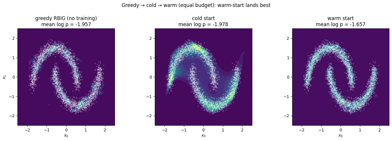
Warm-start delivers the best fit for a fraction of the compute: it inherits RBIG’s data-driven structure and then lets gradients refine the whole stack jointly. This is the bridge the master list calls iterative Gaussianization warm-start — fit greedily, then fine-tune — and it is the practical recipe for parametric Gaussianization at scale: never start a flow from noise when a cheap RBIG fit can put it most of the way there.

Recap¶

start	init NLL	training (3000 steps)	final $\log p$
greedy RBIG	—	none (greedy)	-1.96
cold (random)	$\approx 17$	lr $3\!\times\!10^{-3}$	-1.98
warm (RBIG)	$\approx 2$	lr 10^-3	$\mathbf{-1.66}$ (best)

fit_rbig and gaussianization_flow share a structure, so a greedy fit is a drop-in initialisation for the trainable flow.
At an equal budget the warm start begins where the cold start ends, stays ahead the whole way, and fine-tunes past both the cold flow and the greedy fit.
Fine-tuning uses a moderate LR — a large one-cycle peak would undo the good init.

Next up. We have trained and warm-started flows but read only the final likelihood. 02 — Layer-wise inspection opens a flow up — pushing data through one layer at a time to watch Gaussianity improve and diagnose where in the stack the work happens. (The coupling flow itself — and its warm-start — is the subject of Part 5.)

References¶

Laparra, V., Camps-Valls, G., & Malo, J. (2011). Iterative Gaussianization: From ICA to Random Rotations. IEEE Transactions on Neural Networks, 22(4), 537–549. 10.1109/TNN.2011.2106511