Layer-wise inspection of a Gaussianization flow

02 — Layer-wise inspection of a Gaussianization flow¶

We have trained, warm-started, and compared several flows, always reading just the final log-likelihood. But a Gaussianization flow is a stack of interpretable layers — rotations and marginal transforms — and we can watch the data become Gaussian as it passes through them. Layer-wise inspection answers practical questions: Where does the flow do its work? Are later layers earning their keep? Is the latent actually $\mathcal{N}(0,I)$ , or only in its low-order moments?

A flow’s density direction maps data $x$ to latent $z$ through a composed bijection $T = T_L \circ \cdots \circ T_1$ . We simply apply the $T_k$ one at a time and run the Part 0 diagnostics on each intermediate.

What you will see

The pushforward morph: data → $\mathcal{N}(0,I)$ , snapshot per layer.
The rotation↔marginal push-pull: rotations kill correlation but raise marginal kurtosis; marginal steps Gaussianize it back down.
A diagnosis: the work concentrates early, and a residual kurtosis persists — visible only because we looked inside.
The Scan-unrolling trick for inspecting a gaussianization_flow.

import warnings

warnings.filterwarnings("ignore")

import equinox as eqx
import jax
import jax.numpy as jnp
import jax.random as jr
import matplotlib.pyplot as plt
import numpy as np
from scipy import stats
from sklearn.datasets import make_moons

import gauss_flows as gf
from _style import SCATTER_KW, style_ax

jax.config.update("jax_enable_x64", True)

X, _ = make_moons(n_samples=3000, noise=0.08, random_state=0)
X = jnp.asarray((X - X.mean(0)) / X.std(0))

1. The pushforward, one layer at a time¶

We use a greedy fit_rbig model — a real, well-fit Gaussianization flow whose bijection is an Invert-wrapped Chain, so its layers are directly iterable (no training needed; the same inspection applies to any trained flow, §3). The density map $x\to z$ is the chain’s forward transform; we apply each sub-bijection in turn and keep the intermediate. Each RBIG layer is a pair: a FixedRotation then a MixtureGaussianCDF marginal.

flow = gf.fit_rbig(X, n_layers=6, n_components=8, random_state=0)
layers = flow.bijection.bijection.bijections          # Invert -> Chain -> [rot, marg, rot, marg, ...]
kinds = [type(b).__name__ for b in layers]
print(f"{len(layers)} sub-bijections: {kinds[:4]} ...")

# Apply layers cumulatively; snapshot after each full (rotation + marginal) layer.
A = X
per_step = [np.asarray(A)]                            # after each sub-bijection
for b in layers:
    A = jax.vmap(b.transform)(A)
    per_step.append(np.asarray(A))
layer_snaps = [per_step[0]] + [per_step[i] for i in range(2, len(per_step), 2)]  # input + after each layer

show = [0, 1, 2, 6]
fig, axes = plt.subplots(1, len(show), figsize=(15, 3.7), sharex=True, sharey=True)
for ax, k in zip(axes, show):
    ax.scatter(layer_snaps[k][:, 0], layer_snaps[k][:, 1],
               color=("tab:blue" if k == 0 else "tab:orange"), **SCATTER_KW)
    ax.set(title=("input" if k == 0 else f"after layer {k}"), xlabel="$x_0$" if k == 0 else "$z_0$")
    ax.axhline(0, color="k", lw=0.5); ax.axvline(0, color="k", lw=0.5)
    ax.set_aspect("equal"); style_ax(ax)
fig.suptitle("Pushforward through the flow: two-moons → N(0, I)", y=1.04)
fig.tight_layout()

12 sub-bijections: ['FixedRotation', 'MixtureGaussianCDF', 'FixedRotation', 'MixtureGaussianCDF'] ...

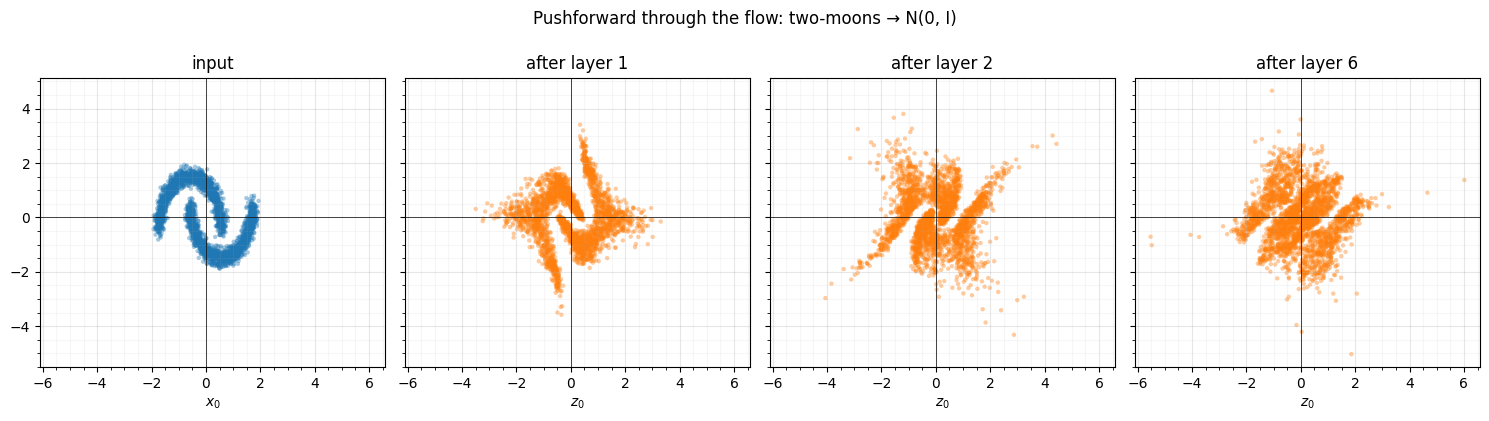
By the first layer the cloud is already close to isotropic, and later layers only polish it — the first hint that the work is front-loaded (the RBIG monotone- reduction property Laparra et al. (2011)). The scatter alone is coarse, though; to see what each sub-step does we need quantitative diagnostics.

2. The rotation↔marginal push-pull¶

We run two Part 0 diagnostics after every sub-bijection: the off-diagonal correlation (dependence) and the mean |excess kurtosis| (marginal non-Gaussianity). Splitting by step type exposes the RBIG mechanism.

A = X
corr, kurt, kind = [], [], []
for b in layers:
    A = jax.vmap(b.transform)(A); Z = np.asarray(A)
    corr.append(abs(np.corrcoef(Z.T)[0, 1]))
    kurt.append(float(np.abs(stats.kurtosis(Z, axis=0)).mean()))
    kind.append("rotation" if type(b).__name__ == "FixedRotation" else "marginal")

x0 = np.abs(np.corrcoef(np.asarray(X).T)[0, 1])
k0 = float(np.abs(stats.kurtosis(np.asarray(X), axis=0)).mean())
print(f"input: corr={x0:.3f}, mean|kurt|={k0:.3f}")
for i, (c, k, t) in enumerate(zip(corr, kurt, kind)):
    print(f"  step {i:2d} [{t:8s}]: corr={c:.3f}  kurt={k:.3f}")

steps = np.arange(1, len(layers) + 1)
is_rot = np.array([t == "rotation" for t in kind])
fig, (axL, axR) = plt.subplots(1, 2, figsize=(12, 4.3))
axL.plot(np.r_[0, steps], np.r_[x0, corr], "-", color="0.6", lw=1, zorder=1)
axL.scatter(steps[is_rot], np.array(corr)[is_rot], color="tab:purple", s=45, label="rotation", zorder=2)
axL.scatter(steps[~is_rot], np.array(corr)[~is_rot], color="tab:green", s=45, label="marginal", zorder=2)
axL.scatter([0], [x0], color="tab:blue", s=45, label="input")
axL.set(title="Correlation: killed by the first rotation", xlabel="sub-bijection", ylabel="|corr|")
axL.legend(fontsize=8); style_ax(axL)

axR.plot(np.r_[0, steps], np.r_[k0, kurt], "-", color="0.6", lw=1, zorder=1)
axR.scatter(steps[is_rot], np.array(kurt)[is_rot], color="tab:purple", s=45, label="rotation (raises kurt)", zorder=2)
axR.scatter(steps[~is_rot], np.array(kurt)[~is_rot], color="tab:green", s=45, label="marginal (lowers kurt)", zorder=2)
axR.scatter([0], [k0], color="tab:blue", s=45, label="input")
axR.set(title="Kurtosis: rotations raise it, marginals knock it down", xlabel="sub-bijection", ylabel="mean |excess kurtosis|")
axR.legend(fontsize=8); style_ax(axR)
fig.tight_layout()

input: corr=0.443, mean|kurt|=1.041
  step  0 [rotation]: corr=0.000  kurt=1.245
  step  1 [marginal]: corr=0.013  kurt=0.014
  step  2 [rotation]: corr=0.000  kurt=0.819
  step  3 [marginal]: corr=0.001  kurt=0.190
  step  4 [rotation]: corr=0.000  kurt=0.781
  step  5 [marginal]: corr=0.016  kurt=0.058
  step  6 [rotation]: corr=0.000  kurt=0.092
  step  7 [marginal]: corr=0.007  kurt=0.233
  step  8 [rotation]: corr=0.000  kurt=0.219
  step  9 [marginal]: corr=0.001  kurt=0.335
  step 10 [rotation]: corr=0.000  kurt=0.748
  step 11 [marginal]: corr=0.002  kurt=0.510

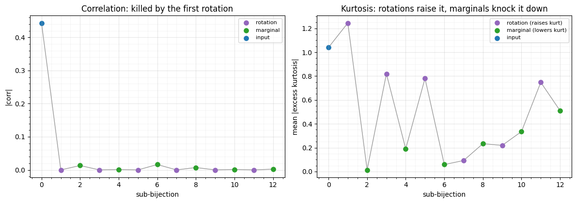
The mechanism is now legible. The first rotation zeroes the correlation and it stays near zero forever (purple/green points hug the axis) — decorrelation is a one-shot job for this 2-D data. Kurtosis tells the richer story: every rotation (purple) raises marginal kurtosis — mixing the axes turns a pair of Gaussian-ish marginals back into something heavier-tailed — and every marginal step (green) knocks it back down. That alternating push-pull is RBIG, seen from the inside.

Two diagnoses fall out. (i) The first layer does the bulk (kurtosis $1.0\to0.01$ , correlation $0.44\to0.01$ ); the remaining layers mostly chase a residual — exactly the redundancy the convergence signal of Part 3 would flag for early-stopping. (ii) A residual kurtosis persists (the final marginals do not fully flatten what the deep rotations stir up), so the latent matches $\mathcal{N}(0,I)$ in mean/variance/correlation but not perfectly in its tails — a limitation you would never see from the log-likelihood alone.

3. Unrolling a `Scan`: inspecting a `gaussianization_flow`¶

fit_rbig gave an iterable Chain. A trainable gaussianization_flow, by contrast, stacks its identical layers in a flowjax Scan (efficient, but its parameters are stored stacked along a leading axis). To inspect it we unroll the Scan into a list of per-layer bijections by indexing that axis, then apply them exactly as above.

def unroll_scan(scan):
    """Split a flowjax Scan into its list of per-layer bijections."""
    template = scan.bijection
    params, static = eqx.partition(template, eqx.is_inexact_array)
    n_layers = jax.tree_util.tree_leaves(params)[0].shape[0]
    return [eqx.combine(jax.tree_util.tree_map(lambda a: a[k], params), static)
            for k in range(n_layers)]

g = gf.gaussianization_flow(jr.key(0), n_dims=2, n_layers=6, n_components=8)
scan = g.bijection.bijection                          # Invert -> Scan
g_layers = unroll_scan(scan)

# Verify: applying the unrolled layers reproduces the full flow's data->latent map.
A = X
for lyr in g_layers:
    A = jax.vmap(lyr.transform)(A)
full = jax.vmap(g.bijection.inverse)(X)
print(f"unrolled {len(g_layers)} layers from the Scan")
print(f"cumulative layers == full flow transform? "
      f"{bool(jnp.allclose(A, full, atol=1e-5))}")
print("=> the same per-layer diagnostics of §2 now apply to any trained flow")

unrolled 6 layers from the Scan
cumulative layers == full flow transform? True
=> the same per-layer diagnostics of §2 now apply to any trained flow

The unrolled layers reproduce the full transform exactly, so everything in §1–§2 — the pushforward morph, the correlation and kurtosis traces — transfers verbatim to a trained gaussianization_flow or coupling_gaussianization_flow. (For the coupling flow each layer also carries a conditioner whose final-kernel magnitude — the zero-kernel contract of Part 5 — is itself a per-layer diagnostic of how “switched on” the coupling is.)

Recap¶

inspection	what it reveals
pushforward morph	data → $\mathcal{N}(0,I)$ ; where the cloud becomes isotropic
correlation per step	rotations decorrelate in one shot
kurtosis per step	rotation raises it, marginal lowers it — the RBIG push-pull
residual kurtosis	latent is Gaussian in low-order moments, not perfectly in tails
`unroll_scan`	per-layer access for a trained `gaussianization_flow`

Looking inside turns “the NLL is -1.96” into “the flow decorrelates instantly, Gaussianizes the marginals over the first layer or two, and leaves a small kurtosis residual” — actionable detail for choosing depth and trusting the latent.

Part 4 → Part 5. That completes parametric Gaussianization flows: NLL training (00), the RBIG warm-start for the diagonal flow (01), and layer-wise inspection (02). The recurring hero is coupling — a bijector whose parameters are predicted by a conditioner network. Part 5 — Coupling-based Gaussianization makes it the headline: the coupling pattern, bijector menu, conditioner architectures and masks — then the diagonal-vs-coupling comparison and the coupling RBIG warm-start (drafted here, but at home there).

References¶

Laparra, V., Camps-Valls, G., & Malo, J. (2011). Iterative Gaussianization: From ICA to Random Rotations. IEEE Transactions on Neural Networks, 22(4), 537–549. 10.1109/TNN.2011.2106511